ROC-AUC Calculator
Receiver Operating Characteristic & AUC analysis • 2026 edition
ROC-AUC Formula:
Show Calculator\( \text{AUC} = \int_0^1 \text{TPR}(FPR) \, dFPR \)
Where:
- \( \text{TPR} = \frac{TP}{TP + FN} \) (True Positive Rate, Sensitivity)
- \( \text{FPR} = \frac{FP}{FP + TN} \) (False Positive Rate)
- \( TP \) = True Positives
- \( FP \) = False Positives
- \( TN \) = True Negatives
- \( FN \) = False Negatives
For discrete points (trapezoidal rule):
- \( \text{AUC} = \sum_{i=1}^{n-1} \frac{\text{TPR}_i + \text{TPR}_{i+1}}{2} \times (\text{FPR}_{i+1} - \text{FPR}_i) \)
- \( \text{AUC} \in [0, 1] \) where 1 is perfect discrimination and 0.5 is random
- \( \text{AUC} > 0.9 \) = Excellent, \( 0.8-0.9 \) = Good, \( 0.7-0.8 \) = Fair, \( < 0.7 \) = Poor
Example: For a model with points at (0.0, 0.0), (0.2, 0.6), (0.6, 0.9), (1.0, 1.0):
\( \text{AUC} = \frac{0.0+0.6}{2} \times (0.2-0.0) + \frac{0.6+0.9}{2} \times (0.6-0.2) + \frac{0.9+1.0}{2} \times (1.0-0.6) \)
\( = 0.3 \times 0.2 + 0.75 \times 0.4 + 0.95 \times 0.4 = 0.06 + 0.30 + 0.38 = 0.74 \)
The model has an AUC of 0.74, indicating fair discriminative ability.
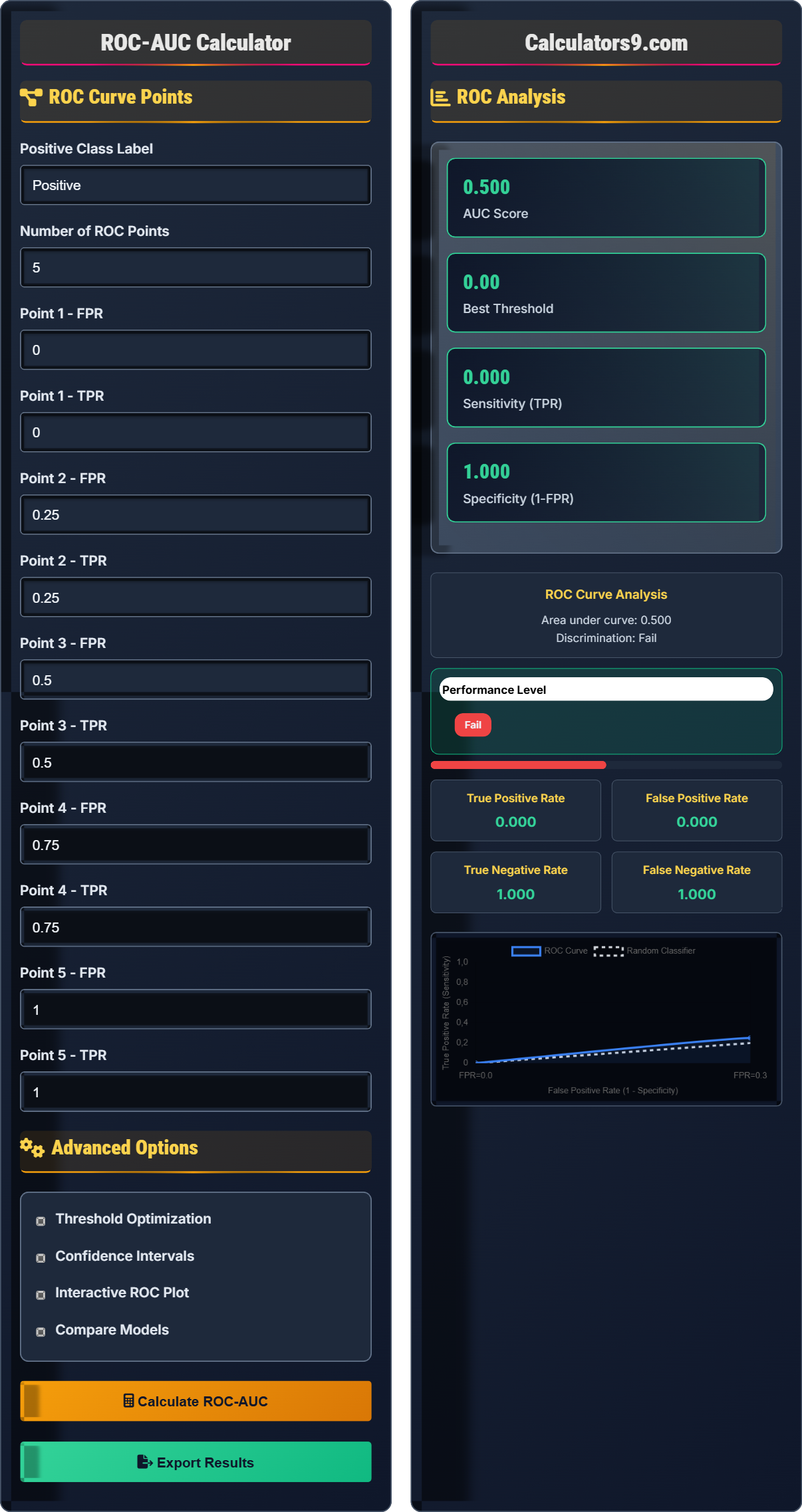
ROC Curve Points
Advanced Options
ROC Analysis
| Metric | Value | Interpretation |
|---|---|---|
| AUC Score | 0.74 | Fair |
| Best Threshold | 0.45 | Optimal for this model |
| Max TPR | 0.90 | High sensitivity |
| Min FPR | 0.20 | Low false positive rate |
Comprehensive ROC-AUC Guide
The ROC (Receiver Operating Characteristic) curve and AUC (Area Under the Curve) are fundamental metrics for evaluating binary classification models. The ROC curve plots True Positive Rate (TPR) against False Positive Rate (FPR) at various threshold settings. The AUC represents the area under this curve, providing a single metric that summarizes the model's ability to distinguish between positive and negative classes.
The AUC calculation using the trapezoidal rule:
Where TPR = True Positive Rate and FPR = False Positive Rate.
ROC-AUC is particularly valuable when:
- Imbalanced datasets: When classes have different distributions
- Threshold independence: When you want to evaluate performance across all thresholds
- Model comparison: When comparing different classification models
- Medical diagnosis: When sensitivity and specificity are both important
- Security applications: When false positive and false negative costs are comparable
- Youden's J Statistic: \( J = \text{TPR} - \text{FPR} \) (maximizes correct classifications)
- Equal Error Rate: Point where FPR = FNR (equal error rates)
- Cost Optimization: Consider domain-specific costs of errors
- Minimum Distance: Minimize distance to top-left corner (0,1)
Metric Fundamentals
Area under the Receiver Operating Characteristic curve.
\( \text{AUC} = \int_0^1 \text{TPR}(FPR) \, dFPR \)
Where TPR=TP/(TP+FN) and FPR=FP/(FP+TN).
- AUC ranges from 0 to 1 (higher is better)
- AUC = 0.5 indicates random performance
- Robust to class imbalance
Model Development
Systematic approach to assessing model effectiveness and reliability.
- Prepare test dataset
- Generate probability scores
- Calculate TPR/FPR at various thresholds
- Plot ROC curve
- Calculate AUC
- Probability calibration
- Threshold selection
- Domain-specific costs
- Statistical significance
ROC-AUC Learning Quiz
What does the ROC curve plot on its axes?
The answer is B) True Positive Rate vs False Positive Rate. The ROC curve plots the True Positive Rate (Sensitivity) on the Y-axis against the False Positive Rate (1 - Specificity) on the X-axis. This allows us to visualize the trade-off between correctly identifying positive cases and incorrectly classifying negative cases as positive across different classification thresholds.
Students must understand that the ROC curve specifically measures the relationship between TPR and FPR. TPR (Sensitivity) measures how well the model identifies positive cases, while FPR measures how often the model incorrectly flags negative cases as positive. The curve shows how these metrics change as the classification threshold varies.
True Positive Rate (TPR): Proportion of actual positives correctly identified
False Positive Rate (FPR): Proportion of actual negatives incorrectly identified as positive
Threshold: Cut-off value for binary classification
• ROC plots TPR vs FPR
• TPR = Sensitivity = TP/(TP+FN)
• FPR = 1 - Specificity = FP/(FP+TN)
• Remember: TPR on Y-axis, FPR on X-axis
• Perfect classifier: TPR=1, FPR=0
• Random classifier: Diagonal line
• Confusing ROC with Precision-Recall curves
• Mixing up TPR and FPR axes
• Forgetting that FPR = 1 - Specificity
Calculate the AUC using the trapezoidal rule for a ROC curve with points: (0,0), (0.2,0.6), (0.6,0.9), (1,1). Show your work.
Using the trapezoidal rule: \( \text{AUC} = \sum_{i=1}^{n-1} \frac{\text{TPR}_i + \text{TPR}_{i+1}}{2} \times (\text{FPR}_{i+1} - \text{FPR}_i) \)
Segment 1: (0,0) to (0.2,0.6)
\( \frac{0 + 0.6}{2} \times (0.2 - 0) = 0.3 \times 0.2 = 0.06 \)
Segment 2: (0.2,0.6) to (0.6,0.9)
\( \frac{0.6 + 0.9}{2} \times (0.6 - 0.2) = 0.75 \times 0.4 = 0.30 \)
Segment 3: (0.6,0.9) to (1,1)
\( \frac{0.9 + 1}{2} \times (1 - 0.6) = 0.95 \times 0.4 = 0.38 \)
Total AUC = 0.06 + 0.30 + 0.38 = 0.74
The AUC is 0.74, indicating fair discriminatory ability.
This calculation demonstrates the trapezoidal rule for approximating the area under the ROC curve. The method breaks the curve into trapezoids and sums their areas. Each segment represents the contribution of that portion of the curve to the total AUC. This approach works well for discrete points obtained from model evaluation.
Trapezoidal Rule: Numerical integration method for area approximation
Area Under Curve: Integral of TPR with respect to FPR
Discriminatory Ability: Model's capability to separate classes
• Use trapezoidal rule for discrete points
• AUC ranges from 0 to 1
• Sum contributions of each segment
• Order points by FPR values
• Include endpoints (0,0) and (1,1)
• Check that AUC is between 0 and 1
• Forgetting to include endpoints
• Not ordering points by FPR
• Arithmetic errors in the calculation
A medical diagnostic test has an AUC of 0.85. If the test is used to screen for a disease that affects 2% of the population, what does this AUC value indicate about the test's performance? How does this compare to a random guess and a perfect test?
AUC Interpretation:
- AUC = 0.85 indicates Good discriminatory ability
- The test can distinguish between diseased and healthy individuals significantly better than random chance
- It correctly ranks a randomly chosen diseased individual higher than a randomly chosen healthy individual 85% of the time
Comparison with other AUC values:
- Random guess (AUC = 0.5): The test has no discriminatory power, equivalent to flipping a coin
- Perfect test (AUC = 1.0): The test perfectly separates diseased and healthy individuals
- Good test (AUC = 0.85): The test performs significantly better than random chance and is clinically useful
For a 2% prevalence disease:
- Out of 1000 people: 20 diseased, 980 healthy
- The test can effectively prioritize which individuals to investigate further
- While not perfect, it significantly reduces the number of false positives compared to random selection
Conclusion: AUC 0.85 represents good performance for medical diagnostics, though clinical decisions would still require additional confirmation.
This example demonstrates how AUC values translate to practical performance. AUC 0.85 means that if you randomly select one diseased and one healthy patient, the test will assign a higher probability of disease to the diseased patient 85% of the time. This interpretation helps connect abstract AUC values to real-world performance.
Discriminatory Ability: Model's capability to separate classes
Prevalence: Proportion of population with condition
Ranking Probability: Relative ordering of predictions
• AUC measures ranking ability, not absolute performance
• Higher AUC indicates better discrimination
• Consider prevalence when interpreting results
• AUC = 0.5 is random performance
• AUC > 0.8 is generally considered good
• AUC > 0.9 is excellent performance
• Confusing AUC with accuracy
• Thinking AUC directly translates to accuracy
• Not considering the clinical context of AUC values
An ROC curve has the following points: (0,0), (0.1,0.4), (0.3,0.7), (0.6,0.9), (0.8,0.95), (1,1). Calculate Youden's J statistic for each point and determine which threshold maximizes it. If missing a positive case (false negative) is 3 times more costly than a false positive, how should this affect threshold selection?
Youden's J Statistic: \( J = \text{TPR} - \text{FPR} \) (maximizes correct classifications)
Calculations for each point:
- Point (0,0): J = 0 - 0 = 0.00
- Point (0.1,0.4): J = 0.4 - 0.1 = 0.30
- Point (0.3,0.7): J = 0.7 - 0.3 = 0.40
- Point (0.6,0.9): J = 0.9 - 0.6 = 0.30
- Point (0.8,0.95): J = 0.95 - 0.8 = 0.15
- Point (1,1): J = 1 - 1 = 0.00
Maximum J occurs at point (0.3, 0.7) with J = 0.40.
Considering cost analysis:
- With FN cost 3x higher than FP cost, we should prioritize higher recall
- This shifts the optimal point toward higher TPR even if FPR increases
- Instead of maximizing J = TPR - FPR, we should maximize: TPR - 3×FPR
- Revised calculations: (0.3,0.7) gives 0.7 - 3×0.3 = -0.2, (0.6,0.9) gives 0.9 - 3×0.6 = -0.9
- At higher cost ratios, we might prefer (0.1,0.4) giving 0.4 - 3×0.1 = 0.1
With FN being 3x more costly, we should select a threshold that prioritizes sensitivity over specificity, likely closer to the (0.1,0.4) point.
This problem demonstrates that optimal threshold selection depends on the cost structure of the application. Youden's J statistic optimizes for equal costs of false positives and negatives. When costs are unequal, we need to adjust our optimization criterion accordingly. This is crucial in real-world applications where different types of errors have different consequences.
Youden's J Statistic: TPR - FPR, maximizes correct classifications
Cost-Sensitive Learning: Optimizing based on error costs
Threshold Optimization: Selecting optimal classification threshold
• Optimal threshold depends on cost structure
• Equal costs: Maximize Youden's J
• Unequal costs: Weight accordingly
• Consider domain-specific costs
• Use cost matrices for optimization
• Evaluate trade-offs at different thresholds
• Using default threshold (0.5) without optimization
• Not considering application-specific costs
• Assuming Youden's J is always optimal
Which of the following is NOT a limitation of ROC-AUC?
The answer is D) Computationally expensive for large datasets. This is NOT a limitation of ROC-AUC. ROC-AUC calculation is actually quite efficient - it requires sorting predictions by probability scores and a single pass through the sorted list to compute the curve points. The other options are genuine limitations: A) ROC-AUC can be overly optimistic for imbalanced datasets, B) AUC doesn't specify the optimal threshold, and C) ROC-AUC is indeed insensitive to class distribution changes (which can be a limitation in some contexts).
Students must understand both the strengths and limitations of ROC-AUC. While it's robust to class imbalance in terms of metric calculation, it can be less informative when the positive class is rare. Also, AUC doesn't tell us which threshold to use in practice - that requires additional analysis based on the specific application requirements.
Class Imbalance: Unequal distribution of classes
Threshold Selection: Choosing optimal classification cutoff
Computational Complexity: Algorithm efficiency measure
• ROC-AUC is computationally efficient
• Consider Precision-Recall for imbalanced data
• AUC doesn't specify optimal threshold
• Use Precision-Recall curves for imbalanced data
• Combine with threshold optimization
• Consider domain-specific metrics
• Thinking ROC-AUC is computationally expensive
• Using ROC-AUC alone for imbalanced datasets
• Not optimizing thresholds for applications
FAQ
Q: What's the difference between ROC-AUC and Precision-Recall AUC, and when should I use each?
A: ROC-AUC and Precision-Recall AUC serve different purposes:
ROC-AUC (True Positive Rate vs False Positive Rate):
- Advantages: Robust to class imbalance, measures ranking ability across all thresholds
- Best for: Balanced datasets, when you care about both positive and negative classes equally
- Formula: \( \text{AUC} = \int_0^1 \frac{\text{TP}}{\text{TP}+\text{FN}} \, d\left(\frac{\text{FP}}{\text{FP}+\text{TN}}\right) \)
- Interpretation: Probability that a positive sample ranks higher than a negative sample
PR-AUC (Precision vs Recall):
- Advantages: More informative for imbalanced datasets, focuses on positive class
- Best for: Highly imbalanced datasets, when positive class is rare
- Formula: \( \text{AUC} = \int_0^1 \frac{\text{TP}}{\text{TP}+\text{FP}} \, d\left(\frac{\text{TP}}{\text{TP}+\text{FN}}\right) \)
- Interpretation: Area under precision-recall curve
Guidelines:
- Use ROC-AUC when: Classes are balanced, both false positives and negatives matter, model comparison
- Use PR-AUC when: Positive class is rare (<10%), precision matters more than false positive rate, cost of false negatives is high
For imbalanced datasets, PR-AUC is generally more informative because it's less optimistic than ROC-AUC.
Q: How do I select the optimal threshold from an ROC curve for practical applications?
A: Several methods exist for threshold selection:
1. Youden's J Statistic:
- Formula: \( J = \text{TPR} - \text{FPR} = \text{Sensitivity} - (1 - \text{Specificity}) \)
- Finds point that maximizes \( \text{TPR} - \text{FPR} \)
- Equivalent to maximizing \( \text{Sensitivity} + \text{Specificity} - 1 \)
- Good when false positive and false negative costs are equal
2. Equal Error Rate (EER):
- Point where FPR = FNR (False Negative Rate)
- Where the ROC curve intersects the line \( \text{TPR} = 1 - \text{FPR} \)
- Equalizes false positive and false negative rates
3. Cost-Based Optimization:
- Consider specific costs: \( C_{FP} \) and \( C_{FN} \)
- Optimize: \( \text{Maximize } \text{TPR} \times C_{TN} - \text{FPR} \times C_{FP} - \text{FNR} \times C_{FN} + \text{TNR} \times C_{TP} \)
- When false negative cost = 3 × false positive cost, use: \( \text{Maximize } \text{TPR} - 3 \times \text{FPR} \)
4. Minimum Distance to Top-Left Corner:
- Minimize: \( \sqrt{(\text{FPR} - 0)^2 + (\text{TPR} - 1)^2} \)
- Point closest to perfect classification (FPR=0, TPR=1)
5. Precision-Recall Based:
- Maximize F1 Score: \( \frac{2 \times \text{Precision} \times \text{Recall}}{\text{Precision} + \text{Recall}} \)
- Useful when precision and recall are both important
Always validate your threshold choice on a held-out test set and consider the practical implications of the chosen threshold in your specific application domain.