AI Model Training Time Estimator
Predict training duration • Resource planning
Model Parameters
Hardware Configuration
Advanced Options
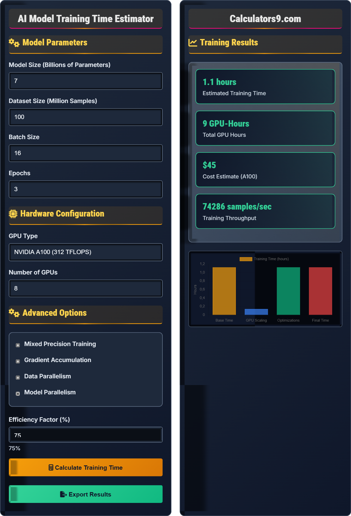
Training Results
| Component | Value | Impact |
|---|---|---|
| Model Parameters | 7B | High |
| Dataset Size | 100M | Medium |
| Hardware | 8×A100 | High |
| Optimizations | Mixed Precision | Positive |
| Resource | Required | Available |
|---|---|---|
| VRAM | 112 GB | 320 GB |
| CPU Cores | 32 cores | 64 cores |
| Memory | 256 GB | 512 GB |
| Storage | 2 TB | 10 TB |
AI Model Training Fundamentals
AI model training is the process of teaching a neural network to recognize patterns and make predictions by feeding it large amounts of data. During training, the model adjusts its internal parameters to minimize prediction errors. The duration of this process depends on multiple factors including model complexity, dataset size, hardware capabilities, and optimization techniques used.
The approximate training time can be calculated using the following formula:
Several techniques can reduce training time while maintaining model quality:
- Mixed Precision Training: Uses FP16 instead of FP32, reducing memory usage and increasing throughput
- Gradient Accumulation: Simulates larger batch sizes without memory constraints
- Data Parallelism: Distributes training across multiple GPUs
- Model Parallelism: Splits large models across multiple devices
- Learning Rate Scheduling: Adjusts learning rate during training for faster convergence
- Estimate VRAM Requirements: Model size + optimizer states + batch data
- Plan for I/O Bottlenecks: Use fast storage and data loading pipelines
- Monitor Efficiency: Track GPU utilization and identify bottlenecks
- Consider Cloud Costs: Balance between training time and computational expense
- Use Spot Instances: Significantly reduce costs for fault-tolerant training
AI Training Time Estimation Quiz
Which of the following factors has the MOST significant impact on AI model training time?
The answer is B) Model parameter count. While all factors contribute to training time, the number of parameters has the most significant impact because it determines the computational complexity of each forward and backward pass. Larger models require exponentially more operations per step.
Understanding the relationship between model size and training time is crucial for AI development planning. The computational complexity grows roughly quadratically with the number of parameters in transformer architectures, making this the dominant factor in training duration.
Parameters: Learnable weights in the neural network that determine model capacity
Forward Pass: Process of computing model output given input
Backward Pass: Process of computing gradients for parameter updates
• Model size scales quadratically with compute requirements
• Larger models require exponentially more training time
• Parameter count is the primary driver of training duration
• Remember: More parameters = More compute time
• Use the square relationship for rough estimates
• Consider model architecture when comparing sizes
• Underestimating the exponential relationship between parameters and compute
• Ignoring the quadratic scaling in transformer models
• Focusing too much on other factors while neglecting model size
Explain how adding more GPUs affects training time and what factors limit perfect scaling. Provide a specific example calculation.
In theory, doubling the number of GPUs should halve the training time through data parallelism. However, several factors prevent perfect scaling:
1. Communication overhead between GPUs (AllReduce operations)
2. Load balancing inefficiencies
3. System bottlenecks (memory, storage, network)
4. Gradient synchronization delays
Example: Training a 7B parameter model takes 48 hours on 8 GPUs. With 16 GPUs, we might expect 24 hours, but due to communication overhead and other factors, it might take 28 hours instead.
Understanding Amdahl's Law is crucial here. As you add more GPUs, the proportion of serial operations (like gradient synchronization) becomes more significant, limiting the potential speedup. The efficiency factor in our calculator accounts for this reality.
Data Parallelism: Distributing identical model copies across multiple GPUs
AllReduce: Collective communication operation for gradient aggregation
Scaling Efficiency: Actual speedup divided by theoretical speedup
• Perfect scaling is rarely achieved in practice
• Communication overhead increases with GPU count
• Efficiency typically decreases as more GPUs are added
• Start with fewer GPUs and scale up gradually
• Monitor GPU utilization to identify bottlenecks
• Consider model parallelism for very large models
• Assuming linear scaling with GPU count
• Not accounting for communication overhead
• Adding too many GPUs without optimizing other bottlenecks
You need to train a 13B parameter model. Training on 8 A100 GPUs takes 72 hours and costs $3,600. Training on 16 A100 GPUs takes 40 hours due to communication overhead but costs $6,400. Which option is more cost-effective if you value your time at $100/hour?
Step 1: Calculate total cost for 8 GPUs option = $3,600 + (72 hours × $100/hour) = $3,600 + $7,200 = $10,800
Step 2: Calculate total cost for 16 GPUs option = $6,400 + (40 hours × $100/hour) = $6,400 + $4,000 = $10,400
Step 3: The 16 GPU option is more cost-effective despite higher compute cost, because it saves 32 hours of your time, valued at $3,200.
Therefore, the 16 GPU option costs $10,400 vs $10,800 for the 8 GPU option, making it $400 cheaper overall.
This problem demonstrates the importance of considering opportunity cost in AI development. While more GPUs cost more in raw compute, they can provide significant value by reducing time-to-market or allowing for more experimentation cycles.
Opportunity Cost: Value of alternative uses of your time
Cost-Effectiveness: Balancing compute cost with time savings
Time-to-Market: Critical factor in competitive AI development
• Total cost = Compute cost + Opportunity cost
• Faster training enables more experiments
• Consider business value of reduced time
• Always factor in time value for business decisions
• Consider iterative development cycles
• Evaluate cloud vs dedicated hardware
• Only considering direct compute costs
• Ignoring the value of accelerated development
• Not accounting for time-sensitive business requirements
You're training a 7B parameter model with mixed precision. Without optimizations, training takes 100 hours on 8 A100 GPUs. With mixed precision, you achieve 2x throughput. With gradient accumulation, you can double the effective batch size without memory constraints. If these optimizations together provide 2.5x speedup, what's the new training time and how does this affect memory requirements?
Step 1: Calculate new training time = Original time ÷ Speedup factor
New time = 100 hours ÷ 2.5 = 40 hours
Step 2: Analyze memory impact:
• Mixed precision (FP16) reduces memory usage by ~50% for parameters
• Gradient accumulation allows larger effective batch sizes without proportional memory increase
• Overall memory efficiency improves significantly
Therefore, training time reduces from 100 to 40 hours (60% reduction) while memory efficiency improves, allowing for larger batch sizes or models.
This demonstrates how optimization techniques can simultaneously improve both time and memory efficiency. Mixed precision training is particularly valuable as it provides both computational speedup and memory savings, enabling larger models or batch sizes.
Mixed Precision: Using FP16 for computations while maintaining FP32 master weights
Gradient Accumulation: Accumulating gradients over multiple mini-batches
Throughput: Samples processed per unit time
• Mixed precision can provide 2x speedup with minimal accuracy loss
• Memory usage scales with batch size and model size
• Optimizations often provide multiplicative benefits
• Always enable mixed precision for modern GPUs
• Use gradient accumulation for memory-constrained scenarios
• Combine optimizations for maximum effect
• Not utilizing mixed precision on modern GPUs
• Ignoring the memory benefits of optimizations
• Underestimating the combined effect of multiple optimizations
When planning resources for training a 175B parameter model, which approach is most practical?
The answer is B) Model parallelism across multiple GPUs. A 175B parameter model requires approximately 350GB of memory just for parameters (assuming FP16). No single consumer GPU has this capacity. Model parallelism distributes the model across multiple devices, making training feasible.
For extremely large models like GPT-3 (175B), neither data parallelism nor single-GPU training is feasible. Model parallelism and pipeline parallelism become necessary techniques. Modern frameworks like Megatron-LM and DeepSpeed provide tools to manage these complex distributed training scenarios.
Model Parallelism: Splitting model layers across multiple devices
Pipeline Parallelism: Staging different model parts across devices
Distributed Training: Coordinating training across multiple machines
• Memory requirements scale linearly with parameters
• Model parallelism is required for very large models
• Communication overhead increases with distribution
• Plan memory requirements before starting training
• Attempting to fit large models on insufficient hardware
• Not accounting for optimizer state memory requirements
• Underestimating communication overhead in distributed training
Training Essentials
Training time scales quadratically with model size and linearly with data.
Time ≈ (Params × Data × Epochs) ÷ (GPU Perf × Parallelism × Eff)
Where Eff accounts for system overhead and optimization efficiency.
- Parameter count dominates training time
- Perfect scaling is impossible
- Memory requirements grow linearly
Optimization Strategies
Reduces memory usage by 50% and increases throughput by 2x.
- Data Parallelism
- Model Parallelism
- Pipeline Parallelism
- Hybrid Approaches
- Communication overhead increases
- Memory bandwidth becomes bottleneck
- System complexity grows
- Debugging becomes harder
FAQ
Q: How does model size affect training time?
A: Training time scales roughly quadratically with model size in transformer architectures. Doubling parameters increases compute by ~4x.
Q: Can I train on multiple GPUs?
A: Yes! But efficiency decreases with more GPUs due to communication overhead. Our calculator accounts for this.