Code Execution Time Estimator
Fast performance analysis • 2026 standards
Execution Time Estimation Formula:
Show the calculatorExecution Time: \( T(n) = C \times f(n) \)
Where:
- \( T(n) \) = estimated execution time
- \( C \) = constant factor (machine dependent)
- \( f(n) \) = complexity function
- \( n \) = input size
Execution time estimation combines algorithmic complexity with hardware performance characteristics. The constant factor C accounts for machine-specific factors like CPU clock speed, memory access patterns, and compiler optimizations. For performance-critical applications, empirical benchmarking is essential to validate estimates.
Example: For O(n²) algorithm with n=1000:
If C = 0.0001 seconds, then T(1000) = 0.0001 × 1000² = 100 seconds
Thus, the estimated execution time is 100 seconds.
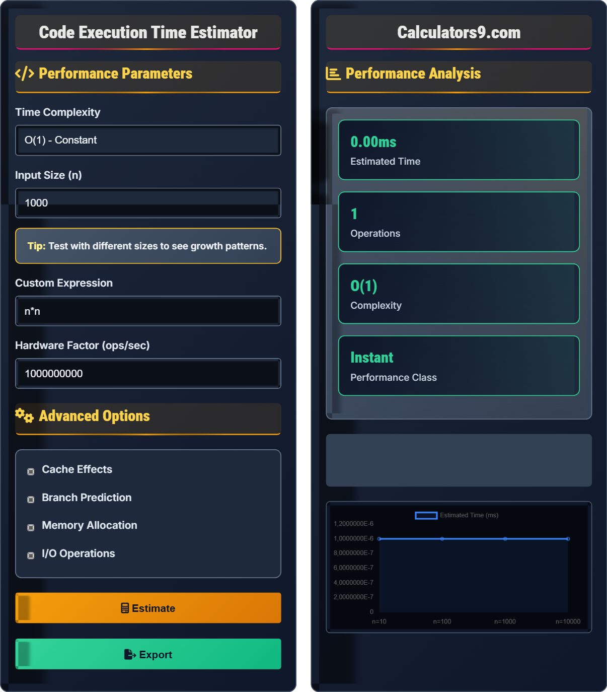
Performance Parameters
Advanced Options
Performance Analysis
| Parameter | Value | Description |
|---|---|---|
| Complexity | O(n²) | Time complexity class |
| Input Size | 1000 | Problem size |
| Operations | 1,000,000 | Estimated operations |
| Hardware | 1.00 GHz | Processing rate |
| Factor | Value | Impact |
|---|---|---|
| Cache Efficiency | 90% | Performance multiplier |
| Memory Allocation | Enabled | Additional overhead |
| I/O Operations | 100 ops | Blocking operations |
| Branch Prediction | Disabled | Conditional overhead |
Comprehensive Performance Guide
Execution time estimation predicts how long a program will take to run based on algorithmic complexity, input size, and hardware characteristics. It combines theoretical algorithm analysis with practical performance factors like cache behavior, memory allocation, and I/O operations. Accurate estimation helps optimize code, allocate resources, and meet performance requirements.
Execution time estimation formula:
Where:
- \( T(n) \) = estimated execution time
- \( C \) = algorithmic constant factor
- \( f(n) \) = complexity function
- \( H \) = hardware multiplier
- \( M \) = memory/cache multiplier
This formula accounts for both algorithmic complexity and hardware-specific factors.
Performance categories based on execution time:
- Instant: < 1ms (real-time interaction)
- Fast: 1-100ms (perceptible delay)
- Acceptable: 100ms-1s (acceptable for most operations)
- Slow: 1-10s (noticeable delay)
- Very Slow: >10s (user abandonment likely)
- Microbenchmarking: Measure small code sections with high precision
- Statistical Profiling: Sample execution over time periods
- Instrumentation: Insert timing code throughout application
- Sampling: Monitor system performance counters
- Simulation: Model performance under different conditions
Performance Fundamentals
Describes the upper bound of an algorithm's growth rate as input size increases.
\( T(n) = C \times f(n) \)
Where C is the constant factor and f(n) is the growth function.
- Focus on dominant terms
- Constants are ignored in Big O
- Practical performance varies by hardware
Optimization Techniques
Improving memory access patterns to maximize cache hit rates.
- Access memory sequentially when possible
- Process data in cache-friendly chunks
- Align data structures to cache lines
- Pre-fetch frequently accessed data
- Profile before optimizing
- Consider algorithmic vs. implementation complexity
- Test with realistic data sets
- Balance readability with performance
Performance Analysis Learning Quiz
Which of the following execution times would be classified as "Acceptable" for user-facing operations?
The answer is B) 500 milliseconds. According to our performance classification, "Acceptable" execution time ranges from 100ms to 1 second. This is the threshold where operations are perceptible but still acceptable for most user interactions.
Understanding performance classes is crucial for user experience design. Operations under 100ms are perceived as instantaneous, while those over 1 second can cause user frustration. The 100ms-1s range represents a sweet spot where users perceive a response but don't feel immediate.
Response Time: Time between user action and system response
Perceived Performance: How fast users think the system is
User Experience: Overall satisfaction with system responsiveness
• <100ms = instantaneous perception
• 100ms-1s = acceptable for most operations
• >1s = noticeable delay
• Use progress indicators for operations >100ms
• Optimize for the 95th percentile response time
• Consider background processing for long operations
• Ignoring user perception thresholds
• Optimizing for average instead of percentiles
• Not testing with realistic data sizes
A sorting algorithm has O(n log n) complexity. If sorting 1000 items takes 0.01 seconds on a particular machine, estimate how long it would take to sort 10,000 items. Show your work.
Given information:
• Time complexity: O(n log n)
• n₁ = 1000, T₁ = 0.01 seconds
• n₂ = 10,000, T₂ = ?
Using the formula T(n) = C × f(n):
0.01 = C × 1000 × log₂(1000)
0.01 = C × 1000 × 9.97
C = 0.01 / (1000 × 9.97) = 1.003 × 10⁻⁶
For n₂ = 10,000:
T₂ = C × 10,000 × log₂(10,000)
T₂ = 1.003 × 10⁻⁶ × 10,000 × 13.29
T₂ ≈ 0.133 seconds
Thus, sorting 10,000 items would take approximately 0.133 seconds.
This problem demonstrates how algorithmic complexity affects performance as input size increases. The O(n log n) complexity means that when the input size increases by a factor of 10, the execution time increases by approximately 10 × (log₂(10) + 1) ≈ 13.3 times. This is much better than O(n²) which would increase by 100 times.
Algorithmic Complexity: Growth rate of resource requirements
Constant Factor: Machine-dependent performance multiplier
Logarithm: Number of times a value can be halved
• Time complexity describes growth patterns
• Constant factors vary by implementation
• Empirical testing validates estimates
• Use log₂(n) ≈ 3.32 × log₁₀(n)
• Remember log₂(1000) ≈ 10
• Test with multiple input sizes to validate
• Forgetting the constant factor in calculations
• Confusing log base (natural vs. binary)
• Not accounting for hardware differences
FAQ
Q: What's the difference between algorithmic complexity and actual execution time?
A: Algorithmic complexity (Big O notation) describes the theoretical growth rate of an algorithm as input size increases, ignoring constants and lower-order terms. Actual execution time depends on many factors including:
- Hardware specifications (CPU, memory, cache)
- Implementation details and compiler optimizations
- System load and other running processes
- Data characteristics (sorted vs. random)
- Memory access patterns and cache effects
Algorithmic complexity provides a framework for comparing algorithms, while actual timing requires empirical measurement.
Q: How can I accurately measure execution time in my code?
A: For accurate timing measurements:
- Run multiple iterations and take the average
- Warm up the JVM/CLR before measuring (for managed languages)
- Use high-resolution timers (nanosecond precision)
- Isolate the code being measured from other operations
- Run tests multiple times and exclude outliers
- Consider using established profiling tools (like JMH for Java)
Also, measure the same operation multiple times and take the minimum time, as this best represents the optimal performance without interference from garbage collection, OS scheduling, etc.