Trend Projection Calculator
Forecast future values • 2026 edition
Trend Projection Formula:
Show the calculator\( \hat{y}_t = \alpha + \beta t + \epsilon_t \)
Where:
- ŷₜ = Projected value at time t
- α = Intercept (baseline value)
- β = Slope (trend coefficient)
- t = Time period
- εₜ = Error term
For exponential smoothing: \( \hat{y}_{t+1} = \alpha y_t + (1-\alpha)\hat{y}_t \)
For polynomial trend: \( \hat{y}_t = a_0 + a_1t + a_2t^2 + ... + a_nt^n \)
This framework allows for various trend modeling approaches depending on data characteristics. The linear model assumes constant rate of change, while polynomial models can capture accelerating or decelerating trends.
Example: If α = 100, β = 5, and t = 12 (months), then ŷ₁₂ = 100 + (5 × 12) = 160
This indicates a projected value of 160 at month 12, assuming a linear trend.
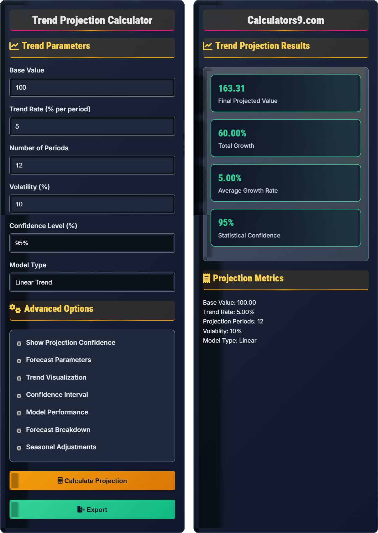
Trend Parameters
Advanced Options
Trend Projection Results
Projection Metrics
Trend Projection Fundamentals
Trend projection is a statistical technique used to forecast future values based on historical data patterns. It identifies consistent patterns in data over time to predict future behavior.
\( \hat{y}_t = \alpha + \beta t + \epsilon_t \)
Where ŷₜ=predicted value, α=intercept, β=slope coefficient, t=time period, εₜ=error term.
- Historical patterns must be stable for accurate projection
- External factors can affect trend continuation
- Confidence intervals reflect prediction uncertainty
- Shorter-term projections are generally more accurate
Model Selection
Different models suit different data patterns: linear for steady trends, exponential for accelerating growth, polynomial for curved patterns.
- Linear: Constant rate of change
- Exponential: Accelerating growth
- Polynomial: Curved trend patterns
- Logarithmic: Slowing growth rate
- Visualize data to identify patterns
- Validate models with historical data
- Consider multiple models for comparison
- Include confidence intervals
Trend Projection Learning Quiz
Which model is most appropriate for projecting a trend that shows accelerating growth?
The answer is B) Exponential model. Exponential models are specifically designed for data that shows accelerating growth, where the rate of change increases over time. The formula y = a × bᵗ captures this accelerating pattern, making it ideal for compound growth scenarios.
Understanding the mathematical characteristics of different models is crucial for accurate forecasting. Linear models assume constant rate of change, logarithmic models show slowing growth, and exponential models capture accelerating growth. The choice of model directly affects the accuracy of projections.
Accelerating Growth: Rate of increase that gets larger over time
Constant Rate: Unchanging rate of change
Exponential Function: Function where variable appears in exponent
• Match model to data pattern characteristics
• Exponential models for compound growth
• Linear models for steady changes
• Plot data to visualize trend patterns
• Use residual analysis to validate model fit
• Consider multiple models for comparison
• Using linear models for exponential growth patterns
• Not validating model assumptions
• Overfitting with complex models
Explain the concept of confidence intervals in trend projection and calculate the 95% confidence interval for a projected value of 150 with a standard error of 10.
Concept: Confidence intervals provide a range of values within which the true value is likely to fall, accounting for uncertainty in the projection.
Calculation:
For 95% confidence interval, use Z-score = 1.96
Lower bound = Projected value - (Z-score × Standard error)
Lower bound = 150 - (1.96 × 10) = 150 - 19.6 = 130.4
Upper bound = Projected value + (Z-score × Standard error)
Upper bound = 150 + (1.96 × 10) = 150 + 19.6 = 169.6
Therefore, the 95% confidence interval is (130.4, 169.6), meaning there's a 95% probability that the true value falls within this range.
Confidence intervals are crucial for understanding the reliability of projections. They acknowledge that projections are estimates with inherent uncertainty. The wider the interval, the greater the uncertainty in the prediction. This helps decision-makers understand the risk associated with relying on projected values.
Confidence Interval: Range of values likely to contain true parameter
Standard Error: Measure of variability in estimate
Statistical Confidence: Probability that interval contains true value
• Confidence intervals reflect prediction uncertainty
• Wider intervals indicate greater uncertainty
• Always report confidence levels with projections
• Use 95% confidence as standard practice
• Consider practical significance of interval width
• Communicate uncertainty to stakeholders
• Not reporting confidence intervals with projections
• Treating point estimates as certain values
• Using inappropriate Z-scores for confidence levels
A company's revenue grew from $1 million to $1.5 million over 5 years. If this trend continues linearly, what would be the projected revenue after 8 years total? What if the growth is exponential instead?
Linear Growth:
Total growth = $1.5M - $1M = $0.5M over 5 years
Annual growth = $0.5M / 5 = $0.1M per year
Revenue after 8 years = $1M + ($0.1M × 8) = $1.8M
Exponential Growth:
Formula: Final = Initial × (1 + r)ⁿ
$1.5M = $1M × (1 + r)⁵
1.5 = (1 + r)⁵
1 + r = 1.5^(1/5) = 1.0845
r = 0.0845 or 8.45% per year
Revenue after 8 years = $1M × (1.0845)⁸ = $1M × 1.925 = $1.925M
Linear projection: $1.8M, Exponential projection: $1.925M
This example demonstrates how model choice significantly affects projections. The exponential model predicts higher growth because it compounds the growth rate each year, while the linear model applies a constant dollar amount each year. This difference becomes more pronounced over longer time horizons.
Linear Growth: Constant amount added each period
Exponential Growth: Constant percentage increase each period
Compounding Effect: Growth on previous growth
• Model choice significantly affects long-term projections
• Exponential growth accelerates over time
• Historical data should inform model selection
• Analyze historical data to identify growth patterns
• Consider sustainability of growth rates
• Validate projections with domain experts
• Assuming exponential growth will continue indefinitely
• Not considering market saturation limits
• Using inappropriate models for data patterns
A retail store's sales show a clear seasonal pattern with Q4 sales 25% higher than average. If the trend projection for December is $120,000, what should the seasonally adjusted forecast be? How would you incorporate this into your projection model?
Seasonal Adjustment Calculation:
Seasonal factor for Q4 = 1 + 0.25 = 1.25
Seasonally adjusted forecast = Projected value / Seasonal factor
Seasonally adjusted forecast = $120,000 / 1.25 = $96,000
Incorporating into Model:
1. Decompose the time series to identify seasonal components
2. Calculate seasonal indices for each period
3. Deseasonalize the data before fitting trend models
4. Apply seasonal factors to trend projections
5. Validate seasonal patterns with historical data
This approach separates trend from seasonal effects for more accurate modeling.
Seasonal adjustment is crucial for accurate forecasting in data with regular patterns. Without accounting for seasonality, trend models may incorrectly interpret seasonal peaks as trend changes. The adjustment process isolates the underlying trend from predictable seasonal variations.
Seasonal Pattern: Regular, predictable variation in data
Seasonal Index: Factor to adjust for seasonal effects
Deseasonalization: Removing seasonal effects from data
• Identify and account for seasonal patterns
• Separate trend from seasonal effects
• Validate seasonal factors with historical data
• Use decomposition methods to identify components
• Apply seasonal factors multiplicatively
• Monitor for changing seasonal patterns
• Not accounting for seasonal variations
• Confusing seasonal patterns with trends
• Using outdated seasonal factors
Which of the following is the most important consideration when validating a trend projection model?
The answer is B) The model accurately predicts out-of-sample data. Out-of-sample validation tests the model's ability to predict future values it hasn't seen before, which is the primary purpose of trend projection. While R-squared measures in-sample fit, out-of-sample accuracy indicates true predictive power.
Model validation is crucial for ensuring projections are reliable. In-sample fit metrics like R-squared can be misleading if the model is overfitted to historical data. Out-of-sample testing, where a portion of data is held back for validation, provides a more realistic assessment of predictive capability.
Out-of-Sample Validation: Testing model on unseen data
In-Sample Fit: How well model fits training data
Overfitting: Model too closely fitted to historical data
• Validate models with out-of-sample data
• Avoid overfitting to historical patterns
• Consider multiple validation metrics
• Use holdout samples for validation
• Cross-validation for robustness testing
• Monitor model performance over time
• Relying solely on in-sample fit metrics
• Not validating predictive capability
• Overfitting complex models to historical data
FAQ
Q: How do I choose the right model for trend projection?
A: The basic linear trend formula is: \( \hat{y}_t = \alpha + \beta t + \epsilon_t \).
Model Selection:
- Linear: \( \hat{y}_t = \alpha + \beta t \) - for constant rate of change
- Exponential: \( \hat{y}_t = \alpha \times \beta^t \) - for compound growth
- Polynomial: \( \hat{y}_t = a_0 + a_1t + a_2t^2 + ... \) - for curved trends
- Logarithmic: \( \hat{y}_t = \alpha + \beta \ln(t) \) - for slowing growth
Plot your data first to identify patterns, then validate models with out-of-sample testing.
Q: What's the importance of confidence intervals in projections?
A: Confidence intervals provide a range of likely values rather than a single point estimate. For example, with a projected value of 150 and standard error of 10:
95% CI = 150 ± (1.96 × 10) = (130.4, 169.6)
This means there's a 95% probability the true value falls between 130.4 and 169.6. Confidence intervals help:
- Assess risk in decision-making
- Understand prediction uncertainty
- Set realistic expectations
- Plan for contingencies
Always consider the width of the interval when making decisions.