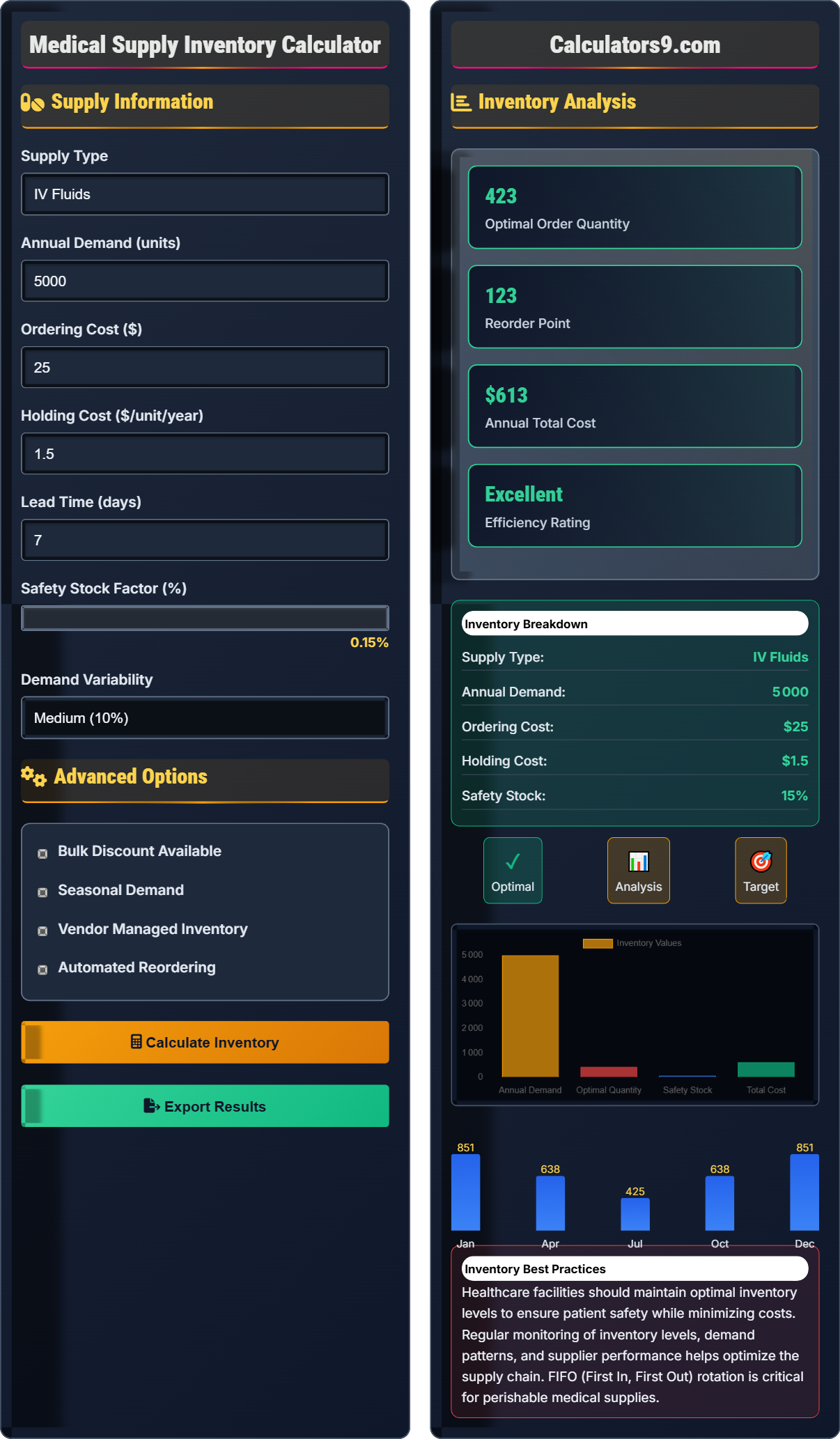
Medical Supply Inventory Calculator
Healthcare operations tool • 2026 edition
Inventory Formula:
Show the calculator\( IQ = \sqrt{\frac{2 \times D \times S}{H}} \times (1 + SSF) \times (1 - DF) \times (1 + RF) \)
Where:
- \( IQ \) = Ideal Quantity (Economic Order Quantity)
- \( D \) = Annual Demand (units per year)
- \( S \) = Ordering Cost per Order ($)
- \( H \) = Holding Cost per Unit per Year ($)
- \( SSF \) = Safety Stock Factor (buffer percentage)
- \( DF \) = Demand Fluctuation Factor (variability reduction)
- \( RF \) = Reorder Factor (lead time consideration)
This formula calculates optimal medical supply inventory levels based on demand, costs, and operational factors. Healthcare facilities should maintain 10-20% safety stock to prevent shortages while avoiding excess inventory. The EOQ model minimizes total inventory costs.
Example: For a supply with \( D = 10,000 \) units/year, \( S = \$50 \) per order, \( H = \$2 \) per unit/year, safety stock factor of 0.15 (15%), demand fluctuation factor of 0.05 (5%), and reorder factor of 0.1 (10%):
\( IQ = \sqrt{\frac{2 \times 10,000 \times 50}{2}} \times (1 + 0.15) \times (1 - 0.05) \times (1 + 0.1) = \sqrt{500,000} \times 1.15 \times 0.95 \times 1.1 = 707.1 \times 1.204 = 851.4 \)
Thus, the optimal order quantity would be 851 units.
Supply Information
Advanced Options
Inventory Analysis
Healthcare facilities should maintain optimal inventory levels to ensure patient safety while minimizing costs. Regular monitoring of inventory levels, demand patterns, and supplier performance helps optimize the supply chain. FIFO (First In, First Out) rotation is critical for perishable medical supplies.
Medical Supply Inventory Framework
Medical supply inventory management follows established inventory control principles adapted for healthcare needs. The Economic Order Quantity (EOQ) model helps minimize total inventory costs while maintaining adequate supply levels. Healthcare facilities must balance cost efficiency with patient safety requirements.
The standard medical supply inventory calculation uses the following formula:
Where:
- \(IQ\) = Ideal Quantity
- \(D\) = Annual Demand
- \(S\) = Ordering Cost per Order
- \(H\) = Holding Cost per Unit per Year
- \(SSF\) = Safety Stock Factor
- \(DF\) = Demand Fluctuation Factor
- \(RF\) = Reorder Factor
Healthcare facilities track various metrics related to supply management:
- IV Fluids: High volume, low cost, strict storage
- Surgical Instruments: High cost, sterilization requirements
- Medications: Expensive, expiry management
- Disposables: Moderate cost, high volume
- Implants: Very high cost, special ordering
- Personal Protective: Critical supply, fluctuating demand
- ABC Analysis: Categorize items by value and frequency
- Vendor-Managed Inventory: Supplier handles stock levels
- Just-In-Time: Receive supplies as needed
- Automated Reordering: System triggers orders
- Centralized Procurement: Bulk purchasing advantages
- Barcoding Systems: Track inventory movement
Inventory Framework
Demand, costs, and safety factors determine optimal inventory levels.
\(IQ = \sqrt{\frac{2 \times D \times S}{H}} \times (1 + SSF) \times (1 - DF) \times (1 + RF)\)
Where IQ=ideal quantity, D=demand, S=ordering cost, H=holding cost, SSF=safety stock factor, DF=demand fluctuation, RF=reorder factor.
- Safety stock: 10-20% of demand
- Reorder point: Lead time × Daily usage
- EOQ minimizes total costs
Inventory Analysis
Supply type, demand patterns, and operational efficiency influence inventory needs.
- Assess annual demand patterns
- Calculate ordering and holding costs
- Determine safety stock requirements
- Calculate optimal order quantities
- High-value items need tighter controls
- Perishable supplies require FIFO rotation
- Seasonal demands affect ordering
Medical Supply Inventory Learning Quiz
What does the Economic Order Quantity (EOQ) model primarily aim to minimize?
The answer is C) Total inventory costs. The EOQ model aims to find the optimal order quantity that minimizes the sum of ordering costs and holding costs. It balances the trade-off between ordering frequently (high ordering costs) and ordering in large quantities (high holding costs).
The EOQ model is a fundamental inventory management concept that demonstrates the trade-off between two opposing costs. As order size increases, ordering costs decrease (fewer orders placed), but holding costs increase (more inventory stored). The optimal point minimizes the total of both costs.
Economic Order Quantity (EOQ): Optimal order size that minimizes total costs
Ordering Costs: Costs associated with placing orders
Holding Costs: Costs of storing inventory
• EOQ minimizes total costs
• Balances ordering vs. holding costs
• Assumes constant demand
• Use EOQ for stable demand items
• Consider safety stock separately
• Monitor demand patterns regularly
• Confusing EOQ with reorder points
• Not accounting for safety stock
• Using EOQ for irregular demand
Calculate the optimal order quantity for a medical supply with annual demand of 8,000 units, ordering cost of $40 per order, and holding cost of $3 per unit per year. Include a 12% safety stock factor. Show your work.
Using the inventory formula: \(IQ = \sqrt{\frac{2 \times D \times S}{H}} \times (1 + SSF)\)
Given:
- D = 8,000 units/year
- S = $40 per order
- H = $3 per unit/year
- SSF = 0.12 (12% safety stock)
Step 1: Calculate EOQ component
EOQ = √[(2 × 8,000 × 40) / 3] = √[640,000 / 3] = √213,333.33 = 461.9
Step 2: Apply safety stock factor
IQ = 461.9 × (1 + 0.12) = 461.9 × 1.12 = 517.3
The optimal order quantity is approximately 517 units.
This calculation demonstrates how the EOQ model works in practice. The square root function ensures that the optimal quantity increases with demand but at a decreasing rate. The safety stock factor provides a buffer above the theoretical optimal quantity to account for uncertainty in demand or supply.
Annual Demand (D): Total units consumed per year
Ordering Cost (S): Fixed cost per order placed
Holding Cost (H): Cost to store one unit for one year
• EOQ = √[(2DS)/H]
• Safety stock is applied as multiplier
• Round to nearest whole unit
• Calculate EOQ component first
• Apply safety stock last
• Verify calculations with examples
• Forgetting to multiply by 2 in numerator
• Misplacing division by holding cost
• Not applying safety stock factor
A hospital uses 1,000 units of IV fluid per week and the supplier takes 5 days to deliver. If the hospital wants to maintain a safety stock equivalent to 2 days of usage, calculate the reorder point. Also calculate how many orders will be placed annually if they order the EOQ of 400 units.
Step 1: Calculate daily usage
Weekly usage = 1,000 units
Daily usage = 1,000 / 7 = 142.86 units/day
Step 2: Calculate reorder point
Reorder Point = (Lead Time × Daily Usage) + Safety Stock
RP = (5 × 142.86) + (2 × 142.86) = 714.3 + 285.7 = 1,000 units
Step 3: Calculate annual orders
Annual demand = 1,000 × 52 = 52,000 units
Number of orders = 52,000 / 400 = 130 orders/year
The reorder point is 1,000 units, and 130 orders will be placed annually.
This example shows how reorder points are calculated to prevent stockouts. The reorder point includes both the lead time demand (to cover the delivery period) and safety stock (to handle demand variability). The number of annual orders depends on the EOQ size relative to total demand.
Reorder Point: Inventory level triggering new order
Lead Time: Time from order placement to deliverySafety Stock: Buffer inventory for uncertainty
• RP = (Lead Time × Daily Usage) + Safety Stock
• Convert weekly to daily usage
• Annual orders = Total demand / Order size
• Always convert to consistent time units
• Include safety stock in reorder point
• Verify daily usage calculation
• Forgetting to convert weekly to daily
• Not including safety stock in RP
• Confusing order size with reorder point
A medical facility orders 500 units of surgical gloves monthly at $2 per unit. Ordering costs are $25 per order, and holding costs are 25% of item value annually. Calculate the annual total inventory cost. Then calculate the savings if they switch to the EOQ model.
Step 1: Calculate parameters
Annual demand (D) = 500 × 12 = 6,000 units
Ordering cost (S) = $25 per order
Holding cost (H) = $2 × 0.25 = $0.50 per unit/year
Current order quantity (Q) = 500 units
Step 2: Calculate current total cost
Number of orders = 6,000 / 500 = 12 orders
Annual ordering cost = 12 × $25 = $300
Average inventory = 500 / 2 = 250 units
Annual holding cost = 250 × $0.50 = $125
Total annual cost = $300 + $125 = $425
Step 3: Calculate EOQ
EOQ = √[(2 × 6,000 × 25) / 0.50] = √[300,000 / 0.50] = √600,000 = 774.6 units
Step 4: Calculate EOQ total cost
Number of orders = 6,000 / 775 = 7.74 ≈ 8 orders
Average inventory = 775 / 2 = 387.5 units
Annual ordering cost = 8 × $25 = $200
Annual holding cost = 387.5 × $0.50 = $193.75
EOQ total cost = $200 + $193.75 = $393.75
Annual savings = $425 - $393.75 = $31.25
This example demonstrates the cost benefits of using EOQ. The current ordering policy (monthly orders of 500 units) results in higher total costs than the EOQ model. The EOQ reduces total costs by finding the optimal balance between ordering and holding costs.
Annual Total Cost: Sum of ordering and holding costs
Cost Analysis: Evaluation of inventory expenses
EOQ Savings: Cost reduction from optimal ordering
• Total cost = Ordering cost + Holding cost
• Ordering cost = (# orders) × (cost per order)
• Holding cost = (average inventory) × (holding cost per unit)
• Calculate all components separately
• Verify EOQ calculation
• Compare before and after costs
• Forgetting to calculate average inventory
• Not rounding EOQ to whole units
• Miscounting number of orders
What is the primary purpose of maintaining safety stock in medical supply inventory?
The answer is B) To protect against stockouts due to demand/supply uncertainty. Safety stock serves as a buffer inventory to handle unexpected increases in demand or delays in supply delivery. In healthcare, this is critical to ensure patient safety and continuity of care.
Safety stock addresses the reality that demand and lead times are not perfectly predictable. In healthcare settings, stockouts can have serious consequences for patient care, making safety stock essential. The level of safety stock depends on the desired service level and the variability in demand and supply.
Safety Stock: Buffer inventory for uncertainty
Stockout: Zero inventory when demand exists
Service Level: Probability of not stockouting
• Safety stock prevents stockouts
• Higher safety stock = higher service level
• Healthcare requires higher safety levels
• Higher uncertainty = higher safety stock
• Critical supplies need more safety stock
• Monitor demand patterns regularly
• Confusing safety stock with reorder point
• Not considering criticality of supplies
• Setting safety stock too low in healthcare
Healthcare Operations FAQ
Q: How does demand variability affect inventory calculations?
A: Demand variability significantly affects inventory calculations through the demand fluctuation factor \( DF \) in our formula: \( IQ = \sqrt{\frac{2 \times D \times S}{H}} \times (1 + SSF) \times (1 - DF) \times (1 + RF) \).
Higher variability requires:
• Increased safety stock (higher SSF)
• More frequent monitoring
• Larger buffer inventories
For example, with high demand variability (DF = 0.20), if annual demand \( D = 10,000 \), ordering cost \( S = \$50 \), holding cost \( H = \$2 \), and safety stock factor \( SSF = 0.25 \):
\( IQ = \sqrt{\frac{2 \times 10,000 \times 50}{2}} \times (1 + 0.25) \times (1 - 0.20) = 707.1 \times 1.25 \times 0.8 = 707.1 \times 1.0 = 707 \) units
This results in maintaining higher inventory levels to accommodate demand fluctuations.
Q: What's the relationship between holding costs and inventory levels?
A: Holding costs are directly proportional to inventory levels. The holding cost component \( H \) in the EOQ formula affects the optimal order quantity inversely:
\( IQ = \sqrt{\frac{2 \times D \times S}{H}} \)
As holding costs increase, the optimal order quantity decreases because it becomes more expensive to maintain large inventories. For a supply with annual demand of 5,000 units and ordering cost of $30:
With low holding cost ($1/unit/year): \( IQ = \sqrt{\frac{2 \times 5,000 \times 30}{1}} = 547.7 \) units
With high holding cost ($3/unit/year): \( IQ = \sqrt{\frac{2 \times 5,000 \times 30}{3}} = 316.2 \) units
Higher holding costs result in smaller, more frequent orders to minimize carrying costs.