ANOVA Calculator
One-way & two-way analysis • 2026 statistics
ANOVA Formula:
Show the calculator\( F = \frac{MS_{between}}{MS_{within}} = \frac{\frac{SS_{between}}{df_{between}}}{\frac{SS_{within}}{df_{within}}} \)
Where:
- \( SS_{between} \) = Sum of squares between groups
- \( SS_{within} \) = Sum of squares within groups
- \( df_{between} \) = Degrees of freedom between groups
- \( df_{within} \) = Degrees of freedom within groups
- \( MS \) = Mean square (Sum of squares divided by degrees of freedom)
ANOVA tests whether the means of three or more groups are significantly different. The F-statistic compares the variation between groups to the variation within groups.
Example: For three groups with sample sizes n₁=5, n₂=5, n₃=5 and means x̄₁=10, x̄₂=12, x̄₃=14:
Total mean: x̄ = (10+12+14)/3 = 12
Between groups SS: 5×[(10-12)² + (12-12)² + (14-12)²] = 5×[4+0+4] = 40
Within groups SS: Σ(sum of squared deviations within each group)
Calculate F = (40/2) / (within groups MS) and compare to critical F-value.
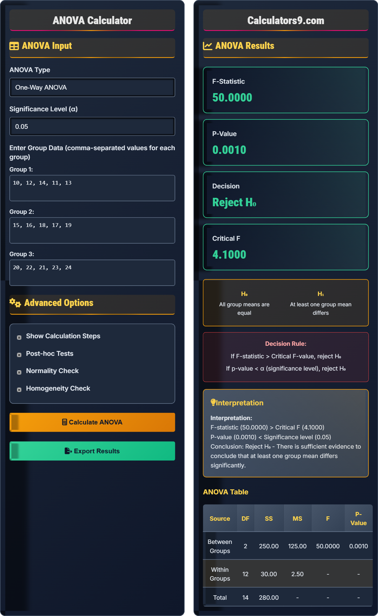
ANOVA Input
Advanced Options
ANOVA Results
H₀
All group means are equal
H₁
At least one group mean differs
Decision Rule:
If F-statistic > Critical F-value, reject H₀
If p-value < α (significance level), reject H₀
ANOVA Table
| Source | DF | SS | MS | F | P-Value |
|---|
Comprehensive ANOVA Guide
Analysis of Variance (ANOVA) is a statistical method used to compare the means of three or more groups simultaneously. It determines whether there are any statistically significant differences between the means of independent groups. ANOVA uses the F-distribution to test hypotheses about population means.
The core ANOVA formula calculates the F-statistic:
Where:
- \( SS_{between} \) = Sum of squares between groups (measures variation between group means)
- \( SS_{within} \) = Sum of squares within groups (measures variation within each group)
- \( df_{between} \) = Degrees of freedom between groups (k-1, where k is number of groups)
- \( df_{within} \) = Degrees of freedom within groups (N-k, where N is total sample size)
- \( MS \) = Mean square (Sum of squares divided by degrees of freedom)
For valid ANOVA results, the following assumptions must be met:
- Independence: Observations within and between groups are independent
- Normality: Data within each group follows a normal distribution
- Homogeneity of Variance: Variances across groups are approximately equal (homoscedasticity)
- Random Sampling: Data collected through random sampling methods
- F-statistic: Ratio of between-group variance to within-group variance. Larger values indicate greater differences between groups
- P-value: Probability of observing the data given that the null hypothesis is true. If p < α, reject H₀
- Degrees of Freedom: Reflect the number of independent pieces of information used in calculation
- Post-hoc Tests: Conducted after significant ANOVA to determine which specific groups differ
ANOVA Fundamentals
Statistical method comparing means of 3+ groups simultaneously.
\(F = \frac{MS_{between}}{MS_{within}}\)
Where F=ratio of between-group to within-group variance.
- Used for 3+ group comparisons
- Tests null hypothesis of equal means
- Requires independence, normality, homogeneity
ANOVA Applications
When comparing means of 3+ groups simultaneously.
- Check assumptions
- Calculate F-statistic
- Compare to critical value
- Interpret p-value
- Reject H₀ if p < α
- Use post-hoc for pairwise comparisons
- Consider effect size (η²)
- Power analysis for sample size
ANOVA Learning Quiz
When is ANOVA most appropriately used?
The answer is B) To compare the means of three or more groups. ANOVA (Analysis of Variance) is specifically designed to test whether there are statistically significant differences between the means of three or more independent groups. While a t-test can compare two groups, ANOVA extends this capability to multiple groups while controlling the overall Type I error rate.
ANOVA stands for Analysis of Variance and is used when we want to compare multiple group means simultaneously. The key advantage over performing multiple t-tests is that ANOVA controls the family-wise error rate, preventing inflation of Type I errors that would occur with multiple comparisons. Think of it as a global test that tells us if at least one group mean is different from the others.
ANOVA: Analysis of Variance - statistical method to compare means of 3+ groups
Type I Error: Incorrectly rejecting a true null hypothesis (false positive)
Family-wise Error Rate: Probability of making at least one Type I error in a set of comparisons
• Use ANOVA for 3+ group comparisons
• Use t-test for 2 group comparisons
• ANOVA controls overall error rate
• Remember: ANOVA = Analysis Of Variance
• Use the mnemonic "ANalysis Of VAriance" to remember its purpose
• ANOVA tells you if differences exist, but not which ones
• Using ANOVA for just two groups (t-test is better)
• Confusing ANOVA with correlation analysis
• Forgetting that ANOVA only tells if differences exist, not which groups differ
Calculate the F-statistic for a one-way ANOVA with the following data: Between-groups mean square (MSB) = 45, Within-groups mean square (MSW) = 15. What does this F-value indicate?
Using the ANOVA formula: F = MSB/MSW
Given:
- MSB (Mean Square Between) = 45
- MSW (Mean Square Within) = 15
Step 1: Calculate F-statistic
F = MSB/MSW = 45/15 = 3.0
Step 2: Interpret the result
An F-value of 3.0 indicates that the variation between groups is 3 times larger than the variation within groups. This suggests there may be significant differences between the group means.
The F-statistic is a ratio that compares the systematic variation (between groups) to the random variation (within groups). When F is close to 1, it suggests that the group means are similar relative to the variability within groups. As F increases above 1, it indicates that the differences between groups are becoming more pronounced compared to the within-group variation.
F-statistic: Ratio of between-group variance to within-group variance
MSB: Mean Square Between groups (systematic variation)
MSW: Mean Square Within groups (random variation)
• F = MSB/MSW
• F > 1 suggests group differences
• Larger F = stronger evidence against H₀
• Remember: F = (Good variation)/(Bad variation)
• Good variation = between groups
• Bad variation = within groups
• Inverting the ratio (MSW/MSB instead of MSB/MSW)
• Misinterpreting F-values close to 1
• Forgetting that F must be positive
A researcher conducts a one-way ANOVA to compare test scores from three different teaching methods. The ANOVA yields an F-statistic of 6.25 with a p-value of 0.003. If the significance level is α = 0.05, what conclusion should be drawn and what should be done next?
Step 1: Compare p-value to significance level
p-value = 0.003 < α = 0.05
Step 2: Make decision
Since p-value < α, we reject the null hypothesis (H₀).
Step 3: State conclusion
There is sufficient evidence to conclude that at least one of the teaching methods produces significantly different test scores compared to the others.
Step 4: Next steps
Because ANOVA only tells us that differences exist (but not which specific groups differ), the researcher should conduct post-hoc tests (such as Tukey's HSD) to determine which specific teaching methods differ from each other.
This example illustrates the two-stage process of ANOVA analysis. First, the omnibus test (ANOVA) determines if any differences exist among the groups. If significant, a second stage is needed to identify which specific pairs of groups differ. This is why ANOVA is called a "global" or "omnibus" test - it gives us a starting point for further investigation.
Omnibus Test: A statistical test that evaluates overall differences without specifying which groups differ
Post-hoc Tests: Follow-up tests conducted after significant ANOVA to identify specific group differences
Null Hypothesis (H₀): All group means are equal
• Reject H₀ if p-value < α
• ANOVA is directional (tests for any difference)
• Post-hoc tests needed for specific comparisons
• Remember: ANOVA tells you "that" differences exist
• Post-hoc tests tell you "which" differences exist
• Always check assumptions before interpreting results
• Concluding which groups differ based on ANOVA alone
• Forgetting to check ANOVA assumptions
• Misinterpreting non-significant results
A researcher wants to compare the effectiveness of 4 different study techniques on exam performance. She randomly assigns 20 students to each technique (total n = 80). Calculate the degrees of freedom for between groups, within groups, and total. Then explain how these values affect the critical F-value.
Given information:
- Number of groups (k) = 4
- Total sample size (N) = 80
- Sample size per group (n) = 20
Step 1: Calculate degrees of freedom between groups
df_between = k - 1 = 4 - 1 = 3
Step 2: Calculate degrees of freedom within groups
df_within = N - k = 80 - 4 = 76
Step 3: Calculate total degrees of freedom
df_total = N - 1 = 80 - 1 = 79
Step 4: Relationship to critical F-value
The critical F-value depends on both df_between and df_within. With df_between = 3 and df_within = 76, the critical F-value at α = 0.05 would be approximately 2.72. Larger df_within generally leads to smaller critical F-values.
Degrees of freedom represent the number of independent pieces of information available for estimation. For between groups, we lose one degree of freedom because the group means must average to the grand mean. For within groups, we lose one degree of freedom per group because each group's deviation is constrained by its mean.
Degrees of Freedom: Number of independent values that can vary in a statistical calculation
df_between: k-1 (number of groups minus 1)
df_within: N-k (total sample size minus number of groups)
• df_between = k - 1
• df_within = N - k
• df_total = N - 1 = df_between + df_within
• Remember: df_between relates to number of groups
• df_within relates to sample size within groups
• Always verify df_total = df_between + df_within
• Confusing the formulas for different types of df
• Forgetting that df_total = df_between + df_within
• Miscounting the number of groups
Which of the following is NOT an assumption of ANOVA?
The answer is D) Equal sample sizes across groups. While equal sample sizes are preferred and make the test more robust, they are not a strict assumption of ANOVA. The three main assumptions of ANOVA are: (1) Independence of observations, (2) Normality of residuals (or normality of populations), and (3) Homogeneity of variances (equal variances across groups). Unequal sample sizes can affect the robustness of the test, especially when variances are also unequal.
It's important to distinguish between assumptions that are required for the validity of the test and those that are preferred but not essential. Independence, normality, and homogeneity are fundamental assumptions that must be met for valid inference. While equal sample sizes are ideal (they maximize power and make the test more robust to violations of homogeneity), ANOVA can still be performed with unequal sample sizes.
Independence: Observations do not influence each other
Homogeneity of Variances: Equal variances across groups (homoscedasticity)
Robustness: Ability of a statistical test to maintain validity despite assumption violations
• Independence is required
• Normality is required
• Homogeneity is required
• Remember: INH for ANOVA assumptions (Independence, Normality, Homogeneity)
• Equal sample sizes are preferred but not required
• Check assumptions with diagnostic plots
• Believing equal sample sizes are required
• Ignoring assumption checks
• Confusing ANOVA assumptions with t-test assumptions
FAQ
Q: What's the difference between one-way and two-way ANOVA, and when should I use each?
A: One-way ANOVA tests the effect of a single independent variable (factor) on a dependent variable across multiple groups. For example, comparing test scores across three different teaching methods.
Two-way ANOVA examines the effects of two independent variables on a dependent variable, including their interaction. For instance, testing how both teaching method AND class size affect test scores, plus whether the effect of teaching method differs by class size.
Use one-way ANOVA when you have one categorical independent variable with 3+ levels. Use two-way ANOVA when you want to examine two factors simultaneously and their potential interaction effect. The formulas expand as follows:
One-way: \( F = \frac{MS_{between}}{MS_{within}} \)
Two-way: Separate F-ratios for Factor A, Factor B, and A×B interaction: \( F_A = \frac{MS_A}{MS_{error}}, F_B = \frac{MS_B}{MS_{error}}, F_{A×B} = \frac{MS_{A×B}}{MS_{error}} \)
Q: How do I interpret ANOVA results when the F-statistic is significant?
A: A significant F-statistic (p < α) means you reject the null hypothesis that all group means are equal. However, ANOVA is an omnibus test - it tells you that differences exist somewhere among the groups, but not which specific groups differ.
After finding a significant result, conduct post-hoc tests such as Tukey's HSD, Bonferroni, or Scheffé to identify which specific group means are significantly different. These tests control for multiple comparisons.
Also consider effect size measures like eta-squared (η² = SS_between / SS_total) to understand the practical significance of your findings. The formula for eta-squared quantifies the proportion of variance in the dependent variable explained by the independent variable(s).