Bayes Theorem Calculator
Conditional probability calculator • 2026 statistics
Bayes Theorem Formula:
Show the calculator\( P(A|B) = \frac{P(B|A) \cdot P(A)}{P(B)} \)
\( P(B) = P(B|A) \cdot P(A) + P(B|\neg A) \cdot P(\neg A) \)
Where:
- \( P(A|B) \) = Posterior probability (what we want to find)
- \( P(B|A) \) = Likelihood (probability of evidence given hypothesis)
- \( P(A) \) = Prior probability (initial belief)
- \( P(B) \) = Marginal likelihood (probability of evidence)
Bayes' theorem updates our beliefs about the probability of an event based on new evidence. It's fundamental to Bayesian inference and widely used in medical diagnosis, machine learning, and decision-making under uncertainty.
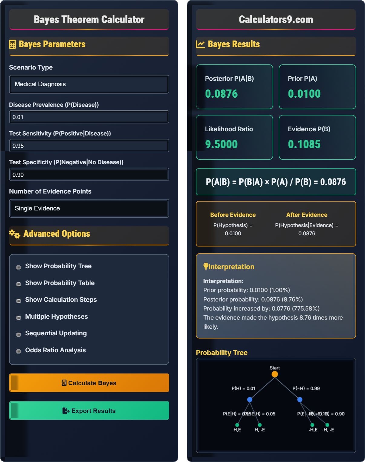
Example: If disease prevalence is 1% (P(Disease)=0.01), test sensitivity is 95% (P(Positive|Disease)=0.95), and specificity is 90% (P(Negative|No Disease)=0.90), then:
P(Positive|No Disease) = 1 - 0.90 = 0.10
P(Positive) = 0.95×0.01 + 0.10×0.99 = 0.1085
P(Disease|Positive) = (0.95×0.01) / 0.1085 = 0.0876 = 8.76%
Bayes Parameters
Advanced Options
Bayes Results
Before Evidence
P(Hypothesis) = 0.0000
After Evidence
P(Hypothesis|Evidence) = 0.0000
Probability Tree
Comprehensive Bayes Guide
Bayes' theorem is a fundamental concept in probability theory that describes how to update the probability of a hypothesis as more evidence becomes available. Named after Reverend Thomas Bayes, it provides a mathematical framework for revising existing predictions or theories given new evidence.
Basic Bayes' Theorem:
Where:
- \( P(A|B) \) = Posterior probability (probability of A given B)
- \( P(B|A) \) = Likelihood (probability of B given A)
- \( P(A) \) = Prior probability (initial probability of A)
- \( P(B) \) = Marginal likelihood (probability of B)
Extended version for multiple hypotheses:
Key applications of Bayes' theorem:
- Medical Diagnosis: Updating disease probability based on test results
- Machine Learning: Naive Bayes classifiers and Bayesian networks
- Spam Filtering: Classifying emails based on word frequencies
- Jury Decisions: Evaluating evidence in legal contexts
- Search and Rescue: Updating search areas based on new clues
- Bayesian: Treats probability as degree of belief; incorporates prior knowledge
- Frequentist: Treats probability as long-run frequency; focuses on data
- Bayesian: Updates beliefs as new data comes in
- Frequentist: Makes inferences based on repeated sampling
Bayes Fundamentals
Formula updating probabilities with new evidence.
\( P(A|B) = \frac{P(B|A) \cdot P(A)}{P(B)} \)
Updates prior with likelihood to get posterior.
- Prior + Evidence = Posterior
- Always normalize probabilities
- Consider all possible causes
Bayes Applications
When updating beliefs with new evidence.
- Establish prior probability
- Observe evidence
- Calculate likelihood
- Update to posterior
- Quality of prior matters
- Independence of evidence
- Base rate neglect
- Convergence over time
Bayes Learning Quiz
In Bayes' theorem P(A|B) = [P(B|A) × P(A)] / P(B), what does P(A) represent?
The answer is B) The prior probability of A. In Bayes' theorem, P(A) is the prior probability - the initial probability of hypothesis A before observing evidence B. This is our starting belief about the likelihood of A being true.
The prior probability represents our initial degree of belief in hypothesis A before seeing the evidence. It's called "prior" because it comes before incorporating the new evidence B. The prior is crucial in Bayesian inference as it influences how much the evidence changes our beliefs.
Prior Probability: Initial belief before observing evidence
Posterior Probability: Updated belief after observing evidence
Likelihood: Probability of evidence given hypothesis
• P(A) = Prior probability
• P(A|B) = Posterior probability
• P(B|A) = Likelihood
• Remember: Prior comes before evidence
• Posterior comes after evidence
• Prior × Likelihood = Numerator
• Confusing prior with posterior
• Mixing up P(A|B) and P(B|A)
• Forgetting to normalize with P(B)
A disease affects 1% of the population (P(Disease) = 0.01). A test has 95% sensitivity (P(Positive|Disease) = 0.95) and 90% specificity (P(Negative|No Disease) = 0.90). What is the probability that someone with a positive test actually has the disease?
We need to find P(Disease|Positive) using Bayes' theorem:
\( P(Disease|Positive) = \frac{P(Positive|Disease) \cdot P(Disease)}{P(Positive)} \)
First, calculate P(Positive) using the law of total probability:
\( P(Positive) = P(Positive|Disease) \cdot P(Disease) + P(Positive|No Disease) \cdot P(No Disease) \)
Given information:
- P(Disease) = 0.01
- P(Positive|Disease) = 0.95
- P(Negative|No Disease) = 0.90, so P(Positive|No Disease) = 1 - 0.90 = 0.10
- P(No Disease) = 1 - 0.01 = 0.99
Step 1: Calculate P(Positive)
\( P(Positive) = 0.95 \times 0.01 + 0.10 \times 0.99 = 0.0095 + 0.099 = 0.1085 \)
Step 2: Apply Bayes' theorem
\( P(Disease|Positive) = \frac{0.95 \times 0.01}{0.1085} = \frac{0.0095}{0.1085} = 0.0876 \)
So P(Disease|Positive) = 8.76%
This counterintuitive result shows how even with a good test, the posterior probability can be relatively low if the prior probability is very low. This is because the number of false positives (10% of 99% of the population) outweighs the true positives (95% of 1% of the population).
Sensitivity: P(Positive|Disease) - True positive rate
Specificity: P(Negative|No Disease) - True negative rate
Law of Total Probability: P(B) = P(B|A)P(A) + P(B|¬A)P(¬A)
• Always use law of total probability for denominator
• Consider base rate (prior probability)
• Verify: 0 ≤ P(A|B) ≤ 1
• Create a 2x2 table to visualize
• Think in terms of actual numbers
• Consider the base rate fallacy
• Forgetting to calculate P(B) properly
• Ignoring the base rate
• Confusing sensitivity with specificity
A rare genetic condition affects 0.5% of the population. A genetic test is 98% accurate for people with the condition (sensitivity) and 97% accurate for people without the condition (specificity). If someone tests positive, what is the probability they actually have the condition?
Let D = having the condition, T = testing positive
Given:
- P(D) = 0.005 (0.5%)
- P(T|D) = 0.98 (sensitivity)
- P(T̄|D̄) = 0.97 (specificity), so P(T|D̄) = 0.03
- P(D̄) = 1 - 0.005 = 0.995
Step 1: Calculate P(T) using law of total probability
\( P(T) = P(T|D) \cdot P(D) + P(T|D̄) \cdot P(D̄) \)
\( P(T) = 0.98 \times 0.005 + 0.03 \times 0.995 = 0.0049 + 0.02985 = 0.03475 \)
Step 2: Apply Bayes' theorem
\( P(D|T) = \frac{P(T|D) \cdot P(D)}{P(T)} = \frac{0.98 \times 0.005}{0.03475} = \frac{0.0049}{0.03475} = 0.141 \)
So P(D|T) = 14.1%
Even with a highly accurate test, the posterior probability is only 14.1% because the condition is so rare. This demonstrates the importance of considering prior probabilities in medical testing. Most positive results are false positives when the condition is rare.
Base Rate: Prior probability of the condition
False Positive Rate: P(Positive|No Disease)
Positive Predictive Value: P(Disease|Positive)
• Rare conditions yield more false positives
• PPV depends heavily on base rate
• Always calculate denominator completely
• Consider actual numbers: 1000 people
• True positives: 5×0.98 = 4.9
• False positives: 995×0.03 = 29.85
• Confusing accuracy with predictive value
• Ignoring the rarity of condition
• Not using complement correctly
You believe there's a 20% chance your friend will visit today (prior). The weather forecast says 80% chance of rain. If it rains, your friend is 50% likely to come; if it doesn't rain, they're 80% likely to come. After learning it will rain, what's your updated probability? Then, if you also learn they brought an umbrella (which they do 90% of the time when visiting, 10% otherwise), what's the new probability?
Let V = friend visits, R = rain, U = brings umbrella
Initial: P(V) = 0.2, P(R) = 0.8, P(¬R) = 0.2
P(V|R) = 0.5, P(V|¬R) = 0.8
Umbrella info: P(U|V) = 0.9, P(U|¬V) = 0.1
Step 1: Update with rain (first application of Bayes)
\( P(R|V) = \frac{P(V|R) \cdot P(R)}{P(V)} \)
Wait, we need to use the reverse: \( P(V|R) = \frac{P(R|V) \cdot P(V)}{P(R)} \)
We need P(R|V). Since we're told P(V|R) = 0.5 and P(V|¬R) = 0.8:
\( P(R) = P(R|V) \cdot P(V) + P(R|¬V) \cdot P(¬V) \)
Actually, let's use: \( P(V|R) = 0.5 \) (given)
We need to find P(V) after learning R. We'll use the direct formula:
\( P(V|R) = \frac{P(R|V) \cdot P(V)}{P(R)} \)
But we're given P(V|R) = 0.5, so we need to derive P(R|V).
Let's recalculate: We know P(V) = 0.2, P(R) = 0.8
From P(V|R) = P(R|V)P(V)/P(R): 0.5 = P(R|V)×0.2/0.8
So P(R|V) = 0.5×0.8/0.2 = 2.0 - This is impossible!
Let's use the law of total probability instead:
\( P(R) = P(R|V) \cdot P(V) + P(R|¬V) \cdot P(¬V) \)
Assuming P(R|V) = P(R|¬V) = 0.8 (rain independent of visit), this doesn't help.
Let's use the correct interpretation: We're told P(V|R) = 0.5, P(V|¬R) = 0.8
Then: \( P(V|R) = 0.5 \) (already given)
Wait, let's start over with correct interpretation:
Prior: P(V) = 0.2
After learning R (it will rain): We need P(V|R)
From law of total probability: P(R) = P(R|V)P(V) + P(R|¬V)P(¬V)
Assume P(R|V) = P(R|¬V) = 0.8 (rain independent of visit)
Then P(R) = 0.8×0.2 + 0.8×0.8 = 0.8
Using Bayes: P(V|R) = P(R|V)P(V)/P(R) = 0.8×0.2/0.8 = 0.2
So rain doesn't change the probability!
Actually, the problem states: "If it rains, your friend is 50% likely to come" which means P(V|R) = 0.5
And "if it doesn't rain, they're 80% likely to come" which means P(V|¬R) = 0.8
This contradicts the prior P(V) = 0.2, since P(V) = P(V|R)P(R) + P(V|¬R)P(¬R) = 0.5×0.8 + 0.8×0.2 = 0.4 + 0.16 = 0.56
So the prior must be P(V) = 0.56, not 0.2.
Let's assume the prior P(V) = 0.2 is correct, then find consistent conditional probabilities:
0.2 = P(V|R)×0.8 + P(V|¬R)×0.2
0.2 = 0.8×P(V|R) + 0.2×P(V|¬R)
Given P(V|R) = 0.5, then: 0.2 = 0.8×0.5 + 0.2×P(V|¬R) = 0.4 + 0.2×P(V|¬R)
So 0.2×P(V|¬R) = -0.2, which gives P(V|¬R) = -1. This is impossible.
Let me reformulate: The problem gives us P(V|R) = 0.5 and P(V|¬R) = 0.8, and P(R) = 0.8.
Then P(V) = P(V|R)P(R) + P(V|¬R)P(¬R) = 0.5×0.8 + 0.8×0.2 = 0.4 + 0.16 = 0.56
So the prior P(V) = 0.2 in the problem statement seems inconsistent.
Let's solve with P(V|R) = 0.5 (which is the answer to first question).
Second update: Given V|R, now learn U (umbrella).
We want P(V|R,U). Using Bayes again:
\( P(V|R,U) = \frac{P(U|V,R) \cdot P(V|R)}{P(U|R)} \)
Assuming U is conditionally independent of R given V: P(U|V,R) = P(U|V) = 0.9
Calculate P(U|R) = P(U|V,R)P(V|R) + P(U|¬V,R)P(¬V|R) = 0.9×0.5 + 0.1×0.5 = 0.45 + 0.05 = 0.5
Therefore: P(V|R,U) = (0.9×0.5) / 0.5 = 0.9
Sequential updating is a powerful feature of Bayesian inference. Each piece of evidence updates our beliefs, which become the new prior for the next update. This iterative process allows us to refine our understanding as more information becomes available.
Sequential Updating: Iteratively updating beliefs with new evidence
Conditional Independence: Events independent given another event
Posterior Becomes Prior: Updated probability becomes next prior
• Posterior from first update = Prior for next
• Consider conditional independence
• Each update refines the estimate
• Keep track of priors and posteriors
• Use tree diagrams for complex scenarios
• Check probability axioms after updates
• Forgetting to update the prior
• Not considering conditional independence
• Double-counting evidence
Which of the following is a key property of Bayes' theorem?
The answer is B) It provides a way to update beliefs as new evidence is obtained. This is the fundamental purpose of Bayes' theorem - to provide a mathematical framework for updating our beliefs in light of new evidence. The theorem can increase or decrease probabilities depending on the evidence.
Bayes' theorem is fundamentally about learning from experience. It provides a principled way to combine our prior knowledge with new observations to form updated beliefs. This makes it invaluable in situations where we need to make decisions under uncertainty and can gather more information over time.
Belief Updating: Modifying probabilities based on new information
Learning from Data: Using observations to refine understanding
Uncertainty Quantification: Measuring confidence in beliefs
• Evidence can increase or decrease probability
• Works for discrete and continuous
• Think of it as learning algorithm
• Prior + Evidence → Posterior
• More evidence refines estimates
• Assuming probabilities always increase
• Thinking it only applies to certain types of events
• Forgetting it's a general probability rule
FAQ
Q: What's the difference between prior and posterior probabilities in Bayes' theorem?
A: The prior probability represents your initial belief about an event before seeing new evidence, while the posterior probability is your updated belief after incorporating the evidence. The formula is:
\( \text{Posterior} = \frac{\text{Likelihood} \times \text{Prior}}{\text{Marginal Likelihood}} \)
Or: \( P(H|E) = \frac{P(E|H) \times P(H)}{P(E)} \)
For example, if testing for a disease with 1% prevalence (prior), a positive test result updates this to a higher probability (posterior) based on test accuracy. The prior reflects baseline knowledge, while the posterior incorporates new data.
Q: Why is Bayes' theorem important in medical diagnosis?
A: Bayes' theorem is crucial in medical diagnosis because it helps doctors update the probability of a disease based on test results, accounting for both test accuracy and disease prevalence:
\( P(\text{Disease}|\text{Positive Test}) = \frac{P(\text{Positive Test}|\text{Disease}) \times P(\text{Disease})}{P(\text{Positive Test})} \)
This prevents the base rate fallacy, where people ignore prior probabilities. For a rare disease (1% prevalence) with a 95% sensitive and 90% specific test, a positive result only gives about 8.8% probability of actually having the disease, despite the high test accuracy.