Chi-Square Calculator
Goodness of fit & independence test • Statistical analysis
Chi-Square Formula:
Show the calculator\( \chi^2 = \sum \frac{(O_i - E_i)^2}{E_i} \)
Where:
- \( O_i \) = Observed frequency for category i
- \( E_i \) = Expected frequency for category i
The chi-square test evaluates whether observed frequencies differ significantly from expected frequencies in categorical data.
Applications: Goodness of fit tests, independence tests in contingency tables, homogeneity tests.
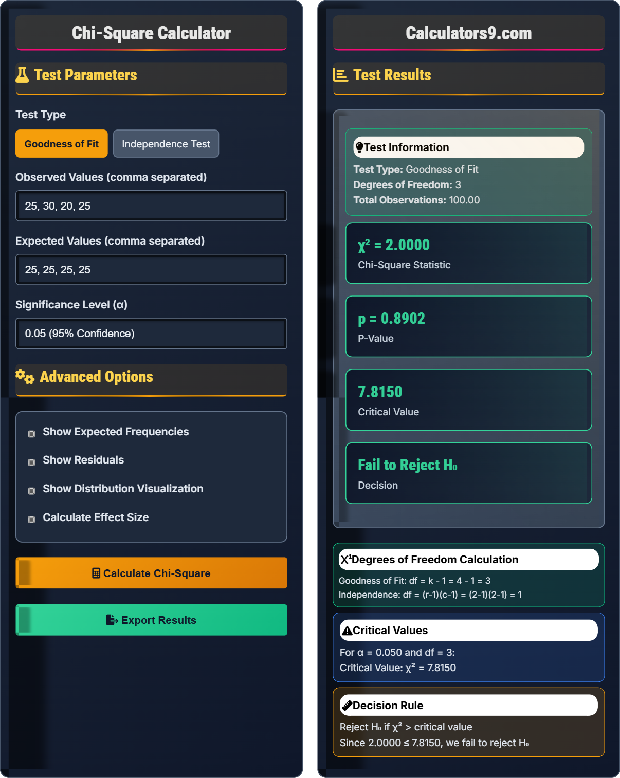
Test Parameters
Advanced Options
Test Results
Test Type: Goodness of Fit
Degrees of Freedom: 3
Total Observations: 100
Goodness of Fit: df = k - 1 = 4 - 1 = 3
Independence: df = (r-1)(c-1) = (2-1)(2-1) = 1
For α = 0.05 and df = 3:
Critical Value: χ² = 9.49
Reject H₀ if χ² > critical value
Since 2.00 ≤ 9.49, we fail to reject H₀
Chi-Square Test Fundamentals
Statistical test used to determine if there's a significant difference between observed and expected frequencies in categorical data.
\( \chi^2 = \sum \frac{(O_i - E_i)^2}{E_i} \)
Where \(O_i\) = observed frequency, \(E_i\) = expected frequency for category i
- Expected frequency should be ≥ 5 for each cell
- Data must be categorical
- Observations must be independent
- Used for goodness of fit and independence tests
Test Types & Applications
Goodness of Fit: Tests if sample data matches a population distribution. Independence: Tests if two categorical variables are related.
- State null and alternative hypotheses
- Calculate expected frequencies
- Compute chi-square statistic
- Determine degrees of freedom
- Find critical value or p-value
- Make decision
- Check expected frequency assumption
- Consider sample size effects
- Report effect size along with p-value
- Interpret practical significance
Chi-Square Testing Learning Quiz
Which of the following is a key assumption for the chi-square test?
The answer is B) Expected frequency should be at least 5 in each cell. One of the key assumptions for the chi-square test is that the expected frequency in each cell should be 5 or greater. This ensures the chi-square distribution provides a good approximation to the test statistic.
The expected frequency assumption is crucial because the chi-square test relies on the chi-square distribution, which is an approximation that becomes more accurate as expected frequencies increase. When expected frequencies are too small, the test becomes unreliable and may lead to incorrect conclusions.
Expected Frequency: Theoretical frequency expected in a cell under the null hypothesis
Observed Frequency: Actual count observed in a cell
Chi-Square Distribution: Probability distribution used in chi-square tests
• Expected frequency ≥ 5 in each cell
• Data must be categorical (nominal or ordinal)
• Observations must be independent
• Combine categories if expected frequencies are too low
• Use Fisher's exact test for small samples
• Applying chi-square to continuous data
• Ignoring expected frequency assumption
• Misinterpreting p-values without considering effect size
A researcher wants to test if gender and preference for a product are independent. The contingency table shows: Male-Like: 40, Male-Dislike: 10, Female-Like: 30, Female-Dislike: 20. At α = 0.05, test for independence.
Step 1: Set up hypotheses
H₀: Gender and product preference are independent
H₁: Gender and product preference are dependent
Step 2: Calculate marginal totals and expected frequencies
Row totals: Male=50, Female=50
Column totals: Like=70, Dislike=30
Grand total: 100
Expected frequencies:
Male-Like: (50×70)/100 = 35
Male-Dislike: (50×30)/100 = 15
Female-Like: (50×70)/100 = 35
Female-Dislike: (50×30)/100 = 15
Step 3: Calculate chi-square statistic
χ² = Σ[(O-E)²/E] = [(40-35)²/35] + [(10-15)²/15] + [(30-35)²/35] + [(20-15)²/15]
= 25/35 + 25/15 + 25/35 + 25/15 = 0.714 + 1.667 + 0.714 + 1.667 = 4.762
Step 4: Determine degrees of freedom
df = (rows-1)(cols-1) = (2-1)(2-1) = 1
Step 5: Find critical value
For α=0.05, df=1: χ²_critical = 3.841
Step 6: Make decision
Since 4.762 > 3.841, we reject H₀
Step 7: Conclusion
There is sufficient evidence to conclude that gender and product preference are dependent at α = 0.05.
This problem demonstrates the independence test where we examine whether two categorical variables are related. The key insight is calculating expected frequencies under the assumption of independence, then comparing observed to expected values using the chi-square formula.
Contingency Table: Cross-tabulation of two categorical variables
Marginal Totals: Row and column sums in contingency table
Independence: Relationship where variables don't influence each other
• df = (rows-1)(cols-1) for independence test
• Expected frequency = (row total × col total) / grand total
• Always check expected frequency assumption
• Draw the contingency table to visualize relationships
• Verify that row/column totals match
• Incorrectly calculating expected frequencies
• Using wrong degrees of freedom formula
• Forgetting to verify expected frequency assumption
FAQ
Q: What's the difference between chi-square goodness of fit and independence tests?
A: The Goodness of Fit test compares observed frequencies in one categorical variable to expected frequencies based on a theoretical distribution:
\( \chi^2 = \sum \frac{(O_i - E_i)^2}{E_i} \)
where df = k - 1 (k = number of categories)
The Independence test examines whether two categorical variables are related using a contingency table:
\( \chi^2 = \sum \frac{(O_{ij} - E_{ij})^2}{E_{ij}} \)
where df = (r-1)(c-1) (r = rows, c = columns)
For goodness of fit: H₀ states that the sample fits a specific distribution. For independence: H₀ states that the two variables are independent.
Both use the same fundamental chi-square formula but differ in how expected frequencies are calculated and what hypotheses are tested.
Q: How do I interpret Cramér's V and when should it be reported?
A: Cramér's V is a measure of association strength for chi-square tests, defined as:
\( V = \sqrt{\frac{\chi^2}{n \cdot \min(r-1, c-1)}} \)
Where n is the total sample size, r is the number of rows, and c is the number of columns.
Interpretation guidelines:
- V = 0: No association between variables
- 0 < V ≤ 0.1: Small effect
- 0.1 < V ≤ 0.3: Medium effect
- V > 0.3: Large effect
For a 2×2 table, Cramér's V is equivalent to the Phi coefficient. Report Cramér's V whenever you conduct a chi-square test to provide context about the practical significance of your findings beyond statistical significance (p-value).
It's especially important when sample sizes are large, as large samples can produce statistically significant results even with trivial associations.