Probability Distribution Calculator
Normal, binomial, poisson distributions • 2026 statistics
Probability Distribution Formulas:
Show the calculatorNormal: \( f(x) = \frac{1}{\sigma\sqrt{2\pi}} e^{-\frac{1}{2}\left(\frac{x-\mu}{\sigma}\right)^2} \)
Binomial: \( P(X=k) = \binom{n}{k} p^k (1-p)^{n-k} \)
Poisson: \( P(X=k) = \frac{\lambda^k e^{-\lambda}}{k!} \)
Where:
- \( \mu \) = Mean of normal distribution
- \( \sigma \) = Standard deviation of normal distribution
- \( n \) = Number of trials (binomial)
- \( p \) = Probability of success (binomial)
- \( \lambda \) = Average rate (poisson)
- \( k \) = Number of successes
Probability distributions model the likelihood of different outcomes in random processes. The normal distribution is continuous and bell-shaped, binomial models discrete success/failure trials, and Poisson models rare events occurring at known average rates.
Example: For a normal distribution with μ=100, σ=15, the probability of X ≤ 115:
Z-score: z = (115-100)/15 = 1
P(X ≤ 115) = P(Z ≤ 1) ≈ 0.8413
For binomial with n=10, p=0.3, probability of exactly 3 successes:
P(X=3) = C(10,3) × 0.3³ × 0.7⁷ = 120 × 0.027 × 0.0824 ≈ 0.2668
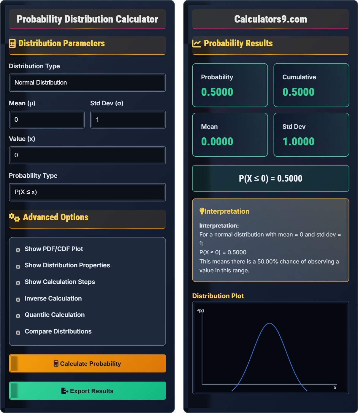
Distribution Parameters
Advanced Options
Probability Results
Distribution Plot
Comprehensive Probability Guide
A probability distribution describes how probabilities are distributed over the values of a random variable. It provides a mathematical function that gives the probabilities of occurrence of different possible outcomes in an experiment. Probability distributions are fundamental to statistical analysis and modeling.
Normal Distribution:
Binomial Distribution:
Poisson Distribution:
Key properties for each distribution:
- Normal: Mean = μ, Variance = σ², Skewness = 0, Kurtosis = 3
- Binomial: Mean = np, Variance = np(1-p), Range = [0, n]
- Poisson: Mean = λ, Variance = λ, Range = [0, ∞]
- Normal: Heights, weights, test scores, measurement errors
- Binomial: Coin flips, survey responses, pass/fail tests
- Poisson: Customer arrivals, defects, accidents, rare events
- General: Risk assessment, quality control, forecasting
Distribution Fundamentals
Function showing likelihood of different outcomes.
\(P(X = x)\) or \(f(x)\) for probability.
Shows likelihood of specific values.
- Probabilities sum to 1
- Continuous: area under curve = 1
- Discrete: sum of all probabilities = 1
Distribution Applications
To model random phenomena and predict outcomes.
- Identify variable type (discrete/continuous)
- Understand underlying process
- Match to appropriate distribution
- Estimate parameters
- Check distribution assumptions
- Validate with data
- Consider parameter uncertainty
- Use goodness-of-fit tests
Probability Learning Quiz
Which probability distribution is most appropriate for modeling the number of customers arriving at a store in one hour, given that on average 15 customers arrive per hour?
The answer is C) Poisson Distribution. The Poisson distribution models the number of events occurring in a fixed interval of time or space at a known average rate. In this case, we're counting the number of customer arrivals (events) in a one-hour time interval with a known average rate (λ = 15).
The Poisson distribution is specifically designed for counting rare events that occur independently at a known average rate. It's characterized by a single parameter λ (lambda), which represents both the mean and variance of the distribution. The Poisson distribution is ideal for modeling arrival processes, defect counts, and other rare event occurrences.
Poisson Distribution: Discrete distribution for counting rare events at known rate
Parameter λ: Average rate of occurrence (mean and variance)
Independence: Events occur independently of each other
• Use Poisson for rare events
• Events must be independent
• Known average rate required
• Think "arrivals" or "occurrences"
• Remember: mean = variance = λ
• Good for low probability, high impact events
• Using normal for count data
• Forgetting independence assumption
• Confusing with binomial distribution
Calculate the probability of exactly 3 successes in 10 trials with a success probability of 0.4 using the binomial formula. Show your work.
Using the binomial formula: \( P(X=k) = \binom{n}{k} p^k (1-p)^{n-k} \)
Given:
- n = 10 (number of trials)
- k = 3 (number of successes)
- p = 0.4 (probability of success)
- (1-p) = 0.6 (probability of failure)
Step 1: Calculate binomial coefficient
\( \binom{10}{3} = \frac{10!}{3!(10-3)!} = \frac{10!}{3! \times 7!} = \frac{10 \times 9 \times 8}{3 \times 2 \times 1} = \frac{720}{6} = 120 \)
Step 2: Calculate probability components
\( p^k = 0.4^3 = 0.064 \)
\( (1-p)^{n-k} = 0.6^7 = 0.0279936 \)
Step 3: Combine all components
\( P(X=3) = 120 \times 0.064 \times 0.0279936 = 0.2150 \)
The binomial coefficient \( \binom{n}{k} \) represents the number of ways to choose k successes from n trials. The formula combines this combinatorial factor with the probability of getting exactly k successes and (n-k) failures. This multiplication principle is fundamental to probability calculations.
Binomial Coefficient: Number of ways to choose k items from n items
Success/Failure Trials: Binary outcomes in each trial
Independent Trials: Outcome of one trial doesn't affect others
• Must have fixed number of trials
• Each trial has 2 outcomes
• Trials must be independent
• Use calculator for large factorials
• Remember: nCk = n!/(k!(n-k)!)
• Check: probabilities sum to 1
• Forgetting the binomial coefficient
• Miscalculating factorials
• Mixing up p and (1-p) exponents
The heights of adult males in a city are normally distributed with mean μ = 70 inches and standard deviation σ = 3 inches. What is the probability that a randomly selected male is taller than 75 inches? Express your answer as a percentage.
Given information:
- Normal distribution: μ = 70, σ = 3
- Find P(X > 75)
Step 1: Calculate Z-score
Z = (X - μ) / σ = (75 - 70) / 3 = 5/3 = 1.67
Step 2: Find P(X > 75) = P(Z > 1.67)
Step 3: Use complement rule
P(Z > 1.67) = 1 - P(Z ≤ 1.67)
From standard normal table, P(Z ≤ 1.67) ≈ 0.9525
Step 4: Calculate final probability
P(X > 75) = 1 - 0.9525 = 0.0475 = 4.75%
The Z-score standardizes the normal distribution by converting raw scores to standard deviations from the mean. This allows us to use the standard normal table. The complement rule P(X > a) = 1 - P(X ≤ a) is often easier than calculating tail probabilities directly.
Z-score: Number of standard deviations from the mean
Standard Normal: Normal distribution with μ=0, σ=1
Complement Rule: P(A) = 1 - P(A')
• Z = (X - μ) / σ
• Use standard normal table
• Apply complement for upper tails
• Draw the normal curve
• Shade the area you want
• Use symmetry when possible
• Forgetting to standardize with Z-score
• Looking up wrong value in table
• Not using complement for upper tails
A call center receives an average of 4 calls per minute. What is the probability that exactly 6 calls will be received in a given minute? Also, what is the probability that fewer than 3 calls will be received in a minute?
Given: λ = 4 calls per minute (Poisson distribution)
Part 1: P(X = 6)
Using Poisson formula: \( P(X=k) = \frac{\lambda^k e^{-\lambda}}{k!} \)
\( P(X=6) = \frac{4^6 e^{-4}}{6!} = \frac{4096 \times e^{-4}}{720} \)
\( e^{-4} \approx 0.0183 \)
\( P(X=6) = \frac{4096 \times 0.0183}{720} = \frac{75.07}{720} = 0.1042 \)
Part 2: P(X < 3) = P(X ≤ 2) = P(X=0) + P(X=1) + P(X=2)
\( P(X=0) = \frac{4^0 e^{-4}}{0!} = \frac{1 \times 0.0183}{1} = 0.0183 \)
\( P(X=1) = \frac{4^1 e^{-4}}{1!} = \frac{4 \times 0.0183}{1} = 0.0733 \)
\( P(X=2) = \frac{4^2 e^{-4}}{2!} = \frac{16 \times 0.0183}{2} = 0.1465 \)
\( P(X < 3) = 0.0183 + 0.0733 + 0.1465 = 0.2381 \)
For "fewer than" probabilities with Poisson, we need to sum individual probabilities. The Poisson distribution has the memoryless property and is particularly useful for modeling rare events occurring at a known average rate. The exponential term e^(-λ) ensures that probabilities sum to 1.
Poisson Process: Events occur independently at constant average rate
Memoryless: Future events independent of past events
Rate Parameter: λ represents average occurrences per interval
• P(X < k) = P(X ≤ k-1)
• Mean = Variance = λ
• Sum all relevant individual probabilities
• Use cumulative tables when available
• Remember: e ≈ 2.71828
• For large λ, normal approximation works
• Forgetting factorial in denominator
• Miscalculating e^(-λ)
• Confusing "less than" with "less than or equal"
Which of the following statements about the normal distribution is TRUE?
The answer is C) Approximately 68% of values lie within one standard deviation of the mean. This is part of the empirical rule (68-95-99.7 rule) for normal distributions: approximately 68% of values fall within 1σ of μ, 95% within 2σ, and 99.7% within 3σ.
The normal distribution is perfectly symmetric, so the mean, median, and mode are all equal. It has zero skewness and is bell-shaped. The empirical rule is a fundamental property that allows quick estimation of probabilities for normally distributed data without complex calculations.
Empirical Rule: 68-95-99.7 rule for normal distribution
• Mean = Median = Mode (symmetric)
• Area under curve = 1
• Empirical rule applies to normal
• Remember: 68-95-99.7
• Draw the bell curve
• Use for quick estimates
• Confusing with skewed distributions
• Forgetting the area equals 1
• Misapplying empirical rule to non-normal data
FAQ
Q: How do I know which probability distribution to use for my data?
A: Choose the distribution based on the characteristics of your data and the process generating it:
- Normal: Continuous data that's approximately symmetric and bell-shaped
- Binomial: Count of successes in n independent trials with constant p
- Poisson: Count of rare events in fixed interval with known average rate
- Exponential: Time between events in a Poisson process
For the normal distribution: \( f(x) = \frac{1}{\sigma\sqrt{2\pi}} e^{-\frac{1}{2}\left(\frac{x-\mu}{\sigma}\right)^2} \)
For binomial: \( P(X=k) = \binom{n}{k} p^k (1-p)^{n-k} \)
For Poisson: \( P(X=k) = \frac{\lambda^k e^{-\lambda}}{k!} \)
Always validate your choice with goodness-of-fit tests.
Q: What's the difference between probability mass function (PMF) and probability density function (PDF)?
A: The PMF gives the probability that a discrete random variable is exactly equal to some value: \( P(X = x) \). The PDF gives the relative likelihood for a continuous random variable to take on a given value, but actual probabilities are found by integrating the PDF over an interval: \( P(a \leq X \leq b) = \int_a^b f(x) dx \).
For discrete distributions (like binomial, Poisson):
\( \sum_{x} P(X = x) = 1 \)
For continuous distributions (like normal):
\( \int_{-\infty}^{\infty} f(x) dx = 1 \)
The PMF gives actual probabilities, while the PDF gives probability densities.