Regression Analysis Tool
Linear & polynomial regression • 2026 statistics
Regression Formula:
Show the calculator\( y = \beta_0 + \beta_1 x + \varepsilon \) (Simple Linear)
\( y = \beta_0 + \beta_1 x + \beta_2 x^2 + \varepsilon \) (Polynomial)
\( R^2 = 1 - \frac{SS_{res}}{SS_{tot}} = 1 - \frac{\sum(y_i - \hat{y}_i)^2}{\sum(y_i - \bar{y})^2} \)
Where:
- \( \beta_0 \) = Y-intercept (constant term)
- \( \beta_1 \) = Slope coefficient
- \( \beta_2 \) = Quadratic coefficient (polynomial)
- \( \varepsilon \) = Error term
- \( R^2 \) = Coefficient of determination
- \( SS_{res} \) = Sum of squares of residuals
- \( SS_{tot} \) = Total sum of squares
Regression analysis models relationships between variables to predict outcomes. The R² value indicates how well the model explains variance in the dependent variable.
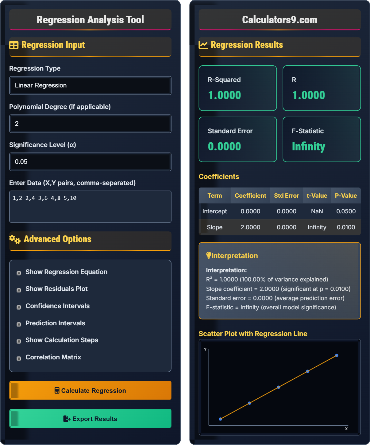
Example: For data points (x,y): (1,2), (2,4), (3,6), (4,8), (5,10):
Mean of y: ȳ = 6
Best fit line: ŷ = 2x
SS_tot = Σ(y_i - ȳ)² = (2-6)² + (4-6)² + ... = 40
SS_res = Σ(y_i - ŷ_i)² = (2-2)² + (4-4)² + ... = 0
R² = 1 - (0/40) = 1.0 (perfect fit)
Regression Input
Advanced Options
Regression Results
Coefficients
| Term | Coefficient | Std Error | t-Value | P-Value |
|---|
Scatter Plot with Regression Line
Comprehensive Regression Guide
Regression analysis is a statistical method used to examine the relationship between a dependent variable (Y) and one or more independent variables (X). It helps predict the value of the dependent variable based on the independent variables. The goal is to find the best-fitting line or curve that represents the relationship between variables.
Simple Linear Regression:
Where:
- \( \beta_0 \) = Y-intercept (value of y when x=0)
- \( \beta_1 \) = Slope (change in y per unit change in x)
- \( \varepsilon \) = Error term (unexplained variation)
For coefficients calculation:
- \( \beta_1 = \frac{\sum(x_i - \bar{x})(y_i - \bar{y})}{\sum(x_i - \bar{x})^2} \)
- \( \beta_0 = \bar{y} - \beta_1 \bar{x} \)
Key metrics for evaluating regression models:
- R-squared (R²): Proportion of variance in dependent variable explained by independent variables (0-1)
- Adjusted R²: R² adjusted for number of predictors in the model
- Standard Error: Average distance of data points from the regression line
- F-statistic: Tests overall significance of the regression model
- P-values: Probability that coefficients are significantly different from zero
- R² close to 1: Model explains most of the variance in the dependent variable
- Low p-values (<0.05): Coefficients are statistically significant
- Residuals plot: Should show random scatter around zero (no pattern)
- Normal probability plot: Residuals should follow normal distribution
- Confidence intervals: Range of likely values for true coefficients
Regression Fundamentals
Statistical method modeling relationships between variables.
\(y = \beta_0 + \beta_1 x + \varepsilon\)
Where y=predicted value, β₀=y-intercept, β₁=slope.
- R² measures model fit (0-1)
- Higher R² = better fit
- Check residuals for randomness
Regression Applications
To predict continuous outcomes based on input variables.
- Identify dependent/independent variables
- Choose regression type
- Fit model
- Evaluate fit
- Check linearity assumption
- Validate residuals
- Consider overfitting
- Use cross-validation
Regression Learning Quiz
What is the primary purpose of regression analysis?
The answer is B) To predict the value of a dependent variable based on independent variables. Regression analysis is primarily used to model and predict the relationship between variables. While correlation measures the strength and direction of a relationship, regression goes further by providing a mathematical equation that allows for prediction of one variable from another.
Regression analysis is fundamentally a predictive modeling technique. It creates a mathematical model that describes how one variable (the dependent variable) changes in response to changes in one or more other variables (independent variables). This model can then be used to make predictions about future observations.
Dependent Variable: The outcome variable being predicted (Y)
Independent Variable: The predictor variable used to predict Y (X)
Regression: Statistical method for modeling relationships and making predictions
• Regression predicts Y from X
• Correlation measures strength of relationship
• Regression provides predictive equations
• Remember: Regression = Prediction
• Independent variables predict dependent variables
• Regression equations allow for forecasting
• Confusing regression with correlation
• Thinking regression proves causation
• Forgetting to validate model assumptions
Calculate the slope coefficient (β₁) for a simple linear regression with the following data: Σ(xᵢ - x̄)(yᵢ - ȳ) = 40, Σ(xᵢ - x̄)² = 20. What does this slope coefficient represent?
Using the formula for slope coefficient: β₁ = Σ(xᵢ - x̄)(yᵢ - ȳ) / Σ(xᵢ - x̄)²
Given:
- Σ(xᵢ - x̄)(yᵢ - ȳ) = 40
- Σ(xᵢ - x̄)² = 20
Step 1: Calculate β₁
β₁ = 40 / 20 = 2.0
Step 2: Interpret the result
The slope coefficient of 2.0 means that for every one-unit increase in the independent variable (X), the dependent variable (Y) increases by 2.0 units on average.
The slope coefficient is the heart of the regression equation. It quantifies the relationship between the independent and dependent variables. A positive slope indicates a positive relationship (as X increases, Y tends to increase), while a negative slope indicates an inverse relationship. The magnitude of the slope tells us the strength of this relationship.
Slope Coefficient (β₁): Change in Y per unit change in X
Y-intercept (β₀): Value of Y when X = 0
Regression Line: Line of best fit through data points
• β₁ = Covariance(X,Y) / Variance(X)
• Positive β₁ = positive relationship
• Magnitude indicates strength of relationship
• Remember: β₁ = rise/run concept
• Units matter: slope has units of Y/X
• Always interpret in context of the problem
• Confusing numerator and denominator in slope formula
• Misinterpreting the sign of the slope
• Forgetting that slope is an average relationship
A researcher performs a regression analysis to predict house prices based on square footage. The model has an R² value of 0.75. How should this R² value be interpreted, and what does it tell us about the model's effectiveness?
Step 1: Understand R² definition
R² = Coefficient of determination = proportion of variance in dependent variable explained by independent variables
Step 2: Interpret the value
R² = 0.75 means that 75% of the variance in house prices is explained by square footage.
Step 3: Evaluate model effectiveness
With R² = 0.75, the model explains a substantial portion of the variability in house prices. This is considered a strong model, though it doesn't account for the remaining 25% of variability which might be due to other factors like location, age, condition, etc.
R² is a key metric for assessing model fit. Values range from 0 to 1, with higher values indicating better fit. However, R² alone doesn't tell the whole story - a model with R² = 0.75 might be excellent for predicting house prices (given the complexity of factors affecting price), while the same R² might be poor for a physics experiment where relationships are more deterministic.
R-squared (R²): Proportion of variance explained by the model (0-1)
Explained Variance: Variability in Y accounted for by X
Unexplained Variance: Remaining variability (residuals)
• R² ranges from 0 to 1
• Higher R² = better fit
• R² doesn't indicate causation
• R² = Explained SS / Total SS
• Adjusted R² penalizes for extra variables
• Context matters for interpretation
• Thinking R² of 1 is always achievable
• Assuming high R² means causation
• Ignoring other model diagnostics
A company has developed a regression model to predict sales based on advertising spend: Sales = 1000 + 2.5×Advertising. If the company plans to spend $10,000 on advertising next month, what sales can they expect? If the actual sales were $36,000, what is the residual?
Given regression equation: Sales = 1000 + 2.5×Advertising
Step 1: Predict sales for $10,000 advertising
Sales = 1000 + 2.5×10,000 = 1000 + 25,000 = $26,000
Step 2: Calculate residual
Residual = Actual - Predicted = $36,000 - $26,000 = $10,000
Step 3: Interpretation
The model underpredicted sales by $10,000. This positive residual indicates that actual sales were higher than the model predicted, suggesting other factors beyond advertising contributed to the increased sales.
Residuals are the differences between observed and predicted values. They represent the portion of the dependent variable that the model fails to explain. Analyzing residuals is crucial for validating regression assumptions and identifying patterns that the model might be missing. A residual of $10,000 suggests that the model systematically underestimated sales in this case.
Residual: Actual value minus predicted value (e = y - ŷ)
Prediction: Using regression equation for new X values
Regression Equation: Mathematical model for prediction
• Residual = Observed - Predicted
• Sum of residuals = 0 (for OLS)
• Residuals should be randomly distributed
• Always check residual plots
• Residuals reveal model inadequacies
• Look for patterns in residuals
• Forgetting to substitute correct X value
• Calculating residual incorrectly
• Ignoring residuals in model evaluation
Which of the following is NOT an assumption of linear regression?
The answer is D) Equal sample sizes across X values. Linear regression does not require equal sample sizes at each X value. The main assumptions of linear regression are: (1) Linearity - the relationship between X and Y is linear, (2) Independence - residuals are independent of each other, (3) Homoscedasticity - constant variance of residuals, and (4) Normality - residuals are normally distributed.
Understanding regression assumptions is crucial for valid inference. Violations of these assumptions can lead to incorrect conclusions. The linearity assumption ensures the model captures the true relationship. Independence ensures that observations don't influence each other. Homoscedasticity ensures constant prediction accuracy across the range of X values. Normality allows for valid hypothesis tests and confidence intervals.
Linearity: Linear relationship between X and Y
Homoscedasticity: Constant variance of residuals
Independence: Residuals are not correlated
• Check assumptions with diagnostic plots
• Violations affect model validity
• Transformations may fix violations
• Remember: LINER (Linearity, Independence, Normality, Equal variance, Random sampling)
• Plot residuals vs fitted values
• Use Q-Q plots for normality check
• Ignoring assumption checks
• Applying regression to non-linear data
• Forgetting to validate with residuals
FAQ
Q: What's the difference between R and R-squared in regression analysis?
A: R (correlation coefficient) measures the strength and direction of the linear relationship between two variables, ranging from -1 to +1. R-squared (coefficient of determination) is the square of R and represents the proportion of variance in the dependent variable explained by the independent variable(s), ranging from 0 to 1.
For example, if R = 0.9, then R² = 0.81, meaning 81% of the variance in Y is explained by X. While R indicates direction (positive/negative) and strength, R² only indicates strength (proportion of explained variance). The formulas are:
\( R = \frac{\sum(x_i - \bar{x})(y_i - \bar{y})}{\sqrt{\sum(x_i - \bar{x})^2 \sum(y_i - \bar{y})^2}} \)
\( R^2 = \left(\frac{\sum(x_i - \bar{x})(y_i - \bar{y})}{\sqrt{\sum(x_i - \bar{x})^2 \sum(y_i - \bar{y})^2}}\right)^2 = \frac{SS_{reg}}{SS_{total}} \)
Q: How do I know if my regression model is good enough?
A: Evaluate your model using multiple criteria:
- R²/Accuracy: Higher values indicate better fit, but context matters
- Residual Analysis: Plot residuals vs fitted values; should show random scatter
- Normality: Residuals should be approximately normally distributed
- Homoscedasticity: Residual variance should be constant across fitted values
- Significance Tests: Coefficients should be statistically significant (p < 0.05)
- Cross-Validation: Test model performance on holdout data
For the standard error of estimate: \( s_e = \sqrt{\frac{SS_{res}}{n-k-1}} \), where n is sample size and k is number of predictors. A smaller standard error indicates more precise predictions.