Integral Simulator
Calculate definite integrals • Numerical methods • Area visualization
Definite Integral Definition:
Show the calculatorDefinition: \( \int_a^b f(x) \, dx = F(b) - F(a) \) (Fundamental Theorem of Calculus)
Numerical Approximation Methods:
- Riemann Sums: \( \sum_{i=1}^{n} f(x_i^*) \Delta x \)
- Trapezoidal Rule: \( \frac{\Delta x}{2}[f(x_0) + 2f(x_1) + \cdots + 2f(x_{n-1}) + f(x_n)] \)
- Simpson's Rule: \( \frac{\Delta x}{3}[f(x_0) + 4f(x_1) + 2f(x_2) + 4f(x_3) + \cdots + f(x_n)] \)
Example: Find \( \int_0^2 x^2 \, dx \) using the trapezoidal rule with n=4.
Step 1: \( \Delta x = \frac{2-0}{4} = 0.5 \)
Step 2: Evaluate function at endpoints: f(0)=0, f(0.5)=0.25, f(1)=1, f(1.5)=2.25, f(2)=4
Step 3: Apply trapezoidal rule: \( \frac{0.5}{2}[0 + 2(0.25) + 2(1) + 2(2.25) + 4] = 0.25[0 + 0.5 + 2 + 4.5 + 4] = 0.25 \times 11 = 2.75 \)
The exact value is \( \frac{x^3}{3} \Big|_0^2 = \frac{8}{3} \approx 2.667 \), so our approximation is quite close.
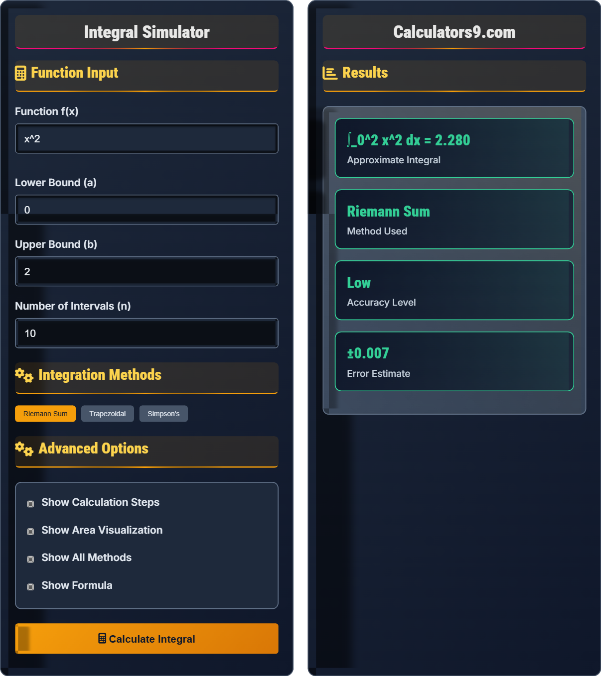
Function Input
Integration Methods
Advanced Options
Results
Comprehensive Integral Guide
Integration is a fundamental operation in calculus that assigns numbers to functions to help describe displacement, area, volume, and other concepts that arise by combining infinitesimal data. The definite integral represents the signed area under a curve between two points. Integration is the reverse process of differentiation, connected by the Fundamental Theorem of Calculus.
The Fundamental Theorem of Calculus establishes the relationship between differentiation and integration:
Where F(x) is an antiderivative of f(x), meaning F'(x) = f(x).
When analytical integration is difficult or impossible, numerical methods approximate definite integrals:
Integration has numerous applications across science and engineering:
- Physics: Work, energy, center of mass
- Engineering: Signal processing, control systems
- Economics: Consumer surplus, total cost
- Biology: Population growth, drug concentration
- More intervals: Generally leads to better accuracy
- Simpson's rule: Most accurate for smooth functions
- Riemann sums: Less accurate but simpler to understand
- Error estimation: Important for numerical reliability
Integral Fundamentals
\( \int_a^b f(x) \, dx \) - Signed area under curve from a to b.
\( \int_a^b f(x) \, dx = F(b) - F(a) \) where F'(x) = f(x).
- Integration reverses differentiation
- Area above x-axis is positive, below is negative
- Definite integral gives a number, indefinite gives a function
Numerical Methods
\( \sum_{i=1}^{n} f(x_i^*) \Delta x \) - Approximate using rectangles.
- Divide interval into n subintervals
- Approximate each segment as trapezoid
- Sum areas of all trapezoids
- More intervals improve accuracy
- Simpson's rule requires even number of intervals
- Higher-order methods better for smooth functions
- Riemann Left: \( \sum_{i=0}^{n-1} f(x_i) \Delta x \)
- Riemann Right: \( \sum_{i=1}^{n} f(x_i) \Delta x \)
- Riemann Midpoint: \( \sum_{i=0}^{n-1} f\left(\frac{x_i + x_{i+1}}{2}\right) \Delta x \)
- Trapezoidal: \( \frac{\Delta x}{2}[f(x_0) + 2f(x_1) + \cdots + f(x_n)] \)
- Simpson's: \( \frac{\Delta x}{3}[f(x_0) + 4f(x_1) + 2f(x_2) + \cdots + f(x_n)] \) (n even)
Integral Learning Quiz
What does the definite integral \( \int_a^b f(x) \, dx \) represent geometrically?
The definite integral \( \int_a^b f(x) \, dx \) represents the signed area under the curve of f(x) between x = a and x = b. Areas above the x-axis count as positive, and areas below the x-axis count as negative.
The slope of the tangent line is related to the derivative, not the integral. The average value of a function over [a,b] is given by \( \frac{1}{b-a} \int_a^b f(x) \, dx \). While integrals can represent distance traveled in physics applications, this is not the geometric interpretation of the integral itself.
The answer is B) The signed area under the curve from a to b.
The geometric interpretation of the definite integral is fundamental to understanding calculus. The "signed" aspect is important - regions above the x-axis contribute positively to the integral, while regions below contribute negatively. This concept connects the abstract mathematical operation to a concrete visual representation.
Definite Integral: A number representing the net area under a curve
Signed Area: Area above x-axis is positive, below is negative
Net Area: The difference between positive and negative areas
• Area above x-axis: positive contribution
• Area below x-axis: negative contribution
• Total integral = positive area - negative area
• Think of integral as "net area"
• Positive regions add to integral, negative subtract
• Symmetric functions around x-axis have integral of 0
• Forgetting that area below x-axis is negative
• Confusing definite integral with antiderivative
• Not accounting for sign changes in the function
Approximate \( \int_0^2 x^2 \, dx \) using a left Riemann sum with n=4 subintervals. Show your work.
Given: f(x) = x², a = 0, b = 2, n = 4
Step 1: Calculate Δx = (b - a)/n = (2 - 0)/4 = 0.5
Step 2: Determine subinterval endpoints: x₀ = 0, x₁ = 0.5, x₂ = 1, x₃ = 1.5, x₄ = 2
Step 3: For left Riemann sum, use left endpoints: x₀, x₁, x₂, x₃
Step 4: Evaluate function at left endpoints:
- f(x₀) = f(0) = 0² = 0
- f(x₁) = f(0.5) = (0.5)² = 0.25
- f(x₂) = f(1) = 1² = 1
- f(x₃) = f(1.5) = (1.5)² = 2.25
Step 5: Apply left Riemann sum formula:
∫₀² x² dx ≈ Δx[f(x₀) + f(x₁) + f(x₂) + f(x₃)]
= 0.5[0 + 0.25 + 1 + 2.25] = 0.5 × 3.5 = 1.75
The left Riemann sum approximation is 1.75.
Riemann sums approximate the area under a curve by dividing the region into rectangles. The left Riemann sum uses the function value at the left endpoint of each subinterval as the height of the rectangle. As the number of rectangles increases, the approximation becomes more accurate. This method provides an intuitive understanding of how integration works.
Riemann Sum: Approximation using rectangular areas
Left Riemann Sum: Uses left endpoints of subintervals
Subinterval: Each of the n equal divisions of [a,b]
• Δx = (b-a)/n (width of each rectangle)
• Left sum: use f(x₀), f(x₁), ..., f(x_{n-1})
• More rectangles = better approximation
• Always sketch the function to visualize rectangles
• Calculate Δx first, then endpoints
• Check that you have n rectangles for n subintervals
• Using wrong number of function evaluations
• Forgetting to multiply by Δx
• Confusing left, right, and midpoint methods
The velocity of a particle moving along a line is given by v(t) = 3t² - 2t + 1, where v is in meters per second and t is in seconds. Find the displacement of the particle from t = 1 to t = 3 seconds. Explain the relationship between velocity and displacement.
Displacement is the integral of velocity with respect to time.
Given: v(t) = 3t² - 2t + 1
Step 1: Set up the integral for displacement: ∫₁³ v(t) dt = ∫₁³ (3t² - 2t + 1) dt
Step 2: Find the antiderivative: ∫(3t² - 2t + 1) dt = t³ - t² + t + C
Step 3: Apply the Fundamental Theorem of Calculus:
∫₁³ (3t² - 2t + 1) dt = [t³ - t² + t]₁³
= (3³ - 3² + 3) - (1³ - 1² + 1)
= (27 - 9 + 3) - (1 - 1 + 1)
= 21 - 1 = 20
The displacement is 20 meters.
Velocity is the rate of change of displacement, so displacement is the accumulation of velocity over time, which is calculated by integration.
This problem demonstrates the fundamental relationship between kinematic quantities: velocity is the derivative of displacement, and displacement is the integral of velocity. This connection between differentiation and integration is a key concept in physics and engineering applications of calculus.
Displacement: Change in position vector
Velocity: Rate of change of displacement
Integration: Accumulation of quantities
• Displacement = ∫ velocity dt
• Velocity = d/dt(displacement)
• Integration accumulates rates of change
• Always include units in physics problems
• Check that your answer makes physical sense
• Remember: integral of rate = accumulation
• Confusing displacement with distance
• Forgetting to evaluate the definite integral properly
• Not applying the Fundamental Theorem of Calculus correctly
The marginal revenue function for selling q items is MR(q) = 100 - 0.2q, where revenue is in dollars. Find the total revenue generated by selling from 100 to 200 items. Explain the relationship between marginal revenue and total revenue.
Total revenue is the integral of marginal revenue with respect to quantity.
Given: MR(q) = 100 - 0.2q
Step 1: Set up the integral: ∫₁₀₀²⁰⁰ MR(q) dq = ∫₁₀₀²⁰⁰ (100 - 0.2q) dq
Step 2: Find the antiderivative: ∫(100 - 0.2q) dq = 100q - 0.1q² + C
Step 3: Apply the Fundamental Theorem of Calculus:
∫₁₀₀²⁰⁰ (100 - 0.2q) dq = [100q - 0.1q²]₁₀₀²⁰⁰
= (100(200) - 0.1(200)²) - (100(100) - 0.1(100)²)
= (20000 - 4000) - (10000 - 1000)
= 16000 - 9000 = 7000
The total revenue generated by selling from 100 to 200 items is $7000.
Marginal revenue is the rate of change of total revenue, so total revenue is the accumulation of marginal revenue, calculated by integration.
In economics, marginal quantities are derivatives of total quantities. Marginal revenue is the derivative of total revenue, so total revenue is the integral of marginal revenue. This relationship is fundamental in economic analysis and optimization problems.
Marginal Revenue: Additional revenue from selling one more unit
Total Revenue: Revenue from selling all units
Marginal Analysis: Study of incremental changes
• Total revenue = ∫ marginal revenue dq
• Marginal revenue = d/dq(total revenue)
• Integration accumulates marginal changes
• Marginal = derivative in economic contexts
• Total = integral of marginal quantity
• Always interpret results economically
• Confusing marginal revenue with average revenue
• Forgetting to calculate the definite integral
• Not interpreting the result in economic terms
Which numerical integration method would likely give the most accurate result for integrating a smooth, rapidly changing function like f(x) = sin(x²) over [0, 2] with a small number of intervals?
For smooth, rapidly changing functions like f(x) = sin(x²), Simpson's rule is typically the most accurate numerical integration method, especially when using a small number of intervals.
Simpson's rule uses quadratic polynomials to approximate the function, making it more accurate than methods that use linear approximations (like the trapezoidal rule) or constant approximations (like Riemann sums). For smooth functions, Simpson's rule can achieve high accuracy even with fewer intervals.
The answer is D) Simpson's rule.
Different numerical integration methods have different orders of accuracy. Riemann sums are O(h), the trapezoidal rule is O(h²), and Simpson's rule is O(h⁴) for smooth functions, where h is the interval width. This means Simpson's rule reduces error much faster as the number of intervals increases, making it superior for smooth functions.
Numerical Integration: Approximating definite integrals computationally
Order of Accuracy: How error decreases with interval size
Smooth Function: Function with continuous derivatives
• Simpson's rule: O(h⁴) for smooth functions
• Trapezoidal rule: O(h²)
• Riemann sums: O(h)
• Use Simpson's rule for smooth functions
• Increase intervals for better accuracy
• Consider function behavior when choosing method
• Using simple methods for complex functions
• Not considering function smoothness
• Forgetting that more intervals improve accuracy
FAQ
Q: What's the difference between definite and indefinite integrals?
A: The key differences are:
Definite integral: \( \int_a^b f(x) \, dx \)
- Has specific upper and lower limits (a and b)
- Evaluates to a specific number (the net area under the curve)
- Represents a quantity with units
Indefinite integral: \( \int f(x) \, dx \)
- Does not have limits of integration
- Evaluates to a function plus a constant (+C)
- Represents a family of functions
The Fundamental Theorem of Calculus connects these concepts: the definite integral can be evaluated using an antiderivative (indefinite integral).
Q: Why do we need numerical integration when we have analytical methods?
A: While analytical integration provides exact answers, numerical integration is necessary in several important scenarios:
1. Non-elementary integrals: Some functions don't have elementary antiderivatives (e.g., \( \int e^{-x^2} dx \), \( \int \frac{\sin x}{x} dx \))
2. Data-driven problems: When we only have discrete data points rather than a formula
3. Complex functions: Analytical integration may be too complex or time-consuming
4. Computational applications: Computer algorithms often use numerical methods
5. Real-world modeling: Functions may be defined by experiments or observations
Numerical methods provide practical solutions when analytical methods fail or aren't feasible.