Matrix Inverse Calculator
Advanced linear algebra tool • Step-by-step solutions
Matrix Inverse Formula:
Show the calculatorFor a 2×2 matrix: \(A^{-1} = \frac{1}{\det(A)} \begin{bmatrix} d & -b \\ -c & a \end{bmatrix}\)
For larger matrices: \(A^{-1} = \frac{1}{\det(A)} \cdot \text{adj}(A)\)
Where adj(A) is the adjugate matrix (transpose of cofactor matrix).
The inverse exists only if the matrix is square and \(\det(A) \neq 0\). The inverse satisfies \(AA^{-1} = A^{-1}A = I\), where I is the identity matrix.
Gauss-Jordan elimination transforms \([A|I]\) into \([I|A^{-1}]\) by applying elementary row operations to convert A into the identity matrix while simultaneously transforming I into A⁻¹.
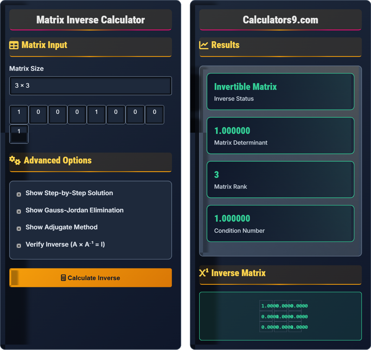
Matrix Input
Advanced Options
Results
Inverse Matrix
Matrix Inverse Fundamentals
The inverse of a square matrix A, denoted A⁻¹, is a matrix such that AA⁻¹ = A⁻¹A = I, where I is the identity matrix. The inverse exists only if the matrix is square and its determinant is non-zero (the matrix is invertible/non-singular). The inverse is unique when it exists.
-
1Definition: AA⁻¹ = A⁻¹A = I
-
2Existence: A⁻¹ exists if and only if det(A) ≠ 0
-
3Uniqueness: If A⁻¹ exists, it is unique
-
4Double Inverse: (A⁻¹)⁻¹ = A
-
5Product Inverse: (AB)⁻¹ = B⁻¹A⁻¹
- Only square matrices can have inverses
- Non-zero determinant is necessary and sufficient
- Inverse of diagonal matrix is diagonal with reciprocals
- (Aᵀ)⁻¹ = (A⁻¹)ᵀ (inverse commutes with transpose)
Calculation Methods
This method forms the augmented matrix [A|I] and performs row operations to transform A into I, resulting in [I|A⁻¹]. It's computationally efficient with O(n³) complexity and numerically stable.
- Gauss-Jordan Elimination: Row reduce [A|I] to [I|A⁻¹]
- Adjugate Method: A⁻¹ = (1/det(A)) × adj(A)
- LU Decomposition: Factor and solve multiple systems
- Cholesky Decomposition: For positive definite matrices
- Gauss-Jordan: O(n³) complexity
- Adjugate method: O(n⁴) complexity
- For large matrices, iterative methods may be preferred
- Numerical stability important for ill-conditioned matrices
Matrix Inverse Learning Quiz
Which of the following statements about matrix inverses is TRUE?
The answer is C) If A and B are invertible, then AB is invertible. This is true because if A and B are invertible, then (AB)⁻¹ = B⁻¹A⁻¹. Statement A is false because only matrices with non-zero determinant are invertible. Statement B is false because inverse matrices can have negative entries. Statement D is false because the inverse of a 2×2 matrix is also 2×2.
This question tests the fundamental understanding of when inverses exist and their properties. It's important to remember that invertibility is determined by the determinant being non-zero, not by the signs of the matrix elements. The product property (AB)⁻¹ = B⁻¹A⁻¹ is a key property that's often confused with the order of multiplication.
Invertible Matrix: A square matrix with non-zero determinant
Singular Matrix: A matrix with zero determinant (no inverse)
Identity Matrix: Matrix I such that AI = IA = A
• Only square matrices can be invertible
• det(A) ≠ 0 is necessary and sufficient for invertibility
• (AB)⁻¹ = B⁻¹A⁻¹ (order matters!)
• Always check if determinant is zero first
• Remember the order reversal in product inverse
• Verify by multiplying A × A⁻¹ = I
• Assuming all square matrices are invertible
• Forgetting the order reversal in (AB)⁻¹
• Confusing inverse with transpose
Find the inverse of the 2×2 matrix: A = \(\begin{bmatrix} 2 & 3 \\ 1 & 4 \end{bmatrix}\). Show your work using the standard formula.
For a 2×2 matrix A = \(\begin{bmatrix} a & b \\ c & d \end{bmatrix}\), the inverse is: A⁻¹ = \(\frac{1}{ad-bc}\begin{bmatrix} d & -b \\ -c & a \end{bmatrix}\)
Step 1: Calculate the determinant
det(A) = ad - bc = (2)(4) - (3)(1) = 8 - 3 = 5
Step 2: Apply the inverse formula
A⁻¹ = \(\frac{1}{5}\begin{bmatrix} 4 & -3 \\ -1 & 2 \end{bmatrix}\)
Step 3: Simplify
A⁻¹ = \(\begin{bmatrix} 4/5 & -3/5 \\ -1/5 & 2/5 \end{bmatrix}\)
Step 4: Verify: A × A⁻¹ = \(\begin{bmatrix} 2 & 3 \\ 1 & 4 \end{bmatrix} \times \begin{bmatrix} 4/5 & -3/5 \\ -1/5 & 2/5 \end{bmatrix} = \begin{bmatrix} 1 & 0 \\ 0 & 1 \end{bmatrix}\)
Therefore, A⁻¹ = \(\begin{bmatrix} 4/5 & -3/5 \\ -1/5 & 2/5 \end{bmatrix}\).
This example demonstrates the straightforward formula for 2×2 matrix inverses. The key insight is that we swap the diagonal elements, change signs of off-diagonal elements, and divide by the determinant. This formula is derived from the general adjugate method but simplified for the 2×2 case.
Adjugate Matrix: Transpose of the cofactor matrix
Cofactor: Signed minor of matrix element
Identity Matrix: Matrix with 1s on diagonal and 0s elsewhere
• Always calculate determinant first
• Division by zero means no inverse exists
• Verify result by multiplication
• Memorize the 2×2 formula: swap diagonals, negate off-diagonals, divide by determinant
• Always verify by multiplying A × A⁻¹ = I
• Check determinant ≠ 0 before proceeding
• Forgetting to divide by the determinant
• Incorrectly changing signs of off-diagonal elements
• Not verifying the result
A system of linear equations can be written as Ax = b where A = \(\begin{bmatrix} 2 & 1 \\ 3 & 4 \end{bmatrix}\) and b = \(\begin{bmatrix} 5 \\ 11 \end{bmatrix}\). Find the solution vector x using the matrix inverse. What is the solution?
Step 1: Find the inverse of A
det(A) = (2)(4) - (1)(3) = 8 - 3 = 5
A⁻¹ = \(\frac{1}{5}\begin{bmatrix} 4 & -1 \\ -3 & 2 \end{bmatrix} = \begin{bmatrix} 4/5 & -1/5 \\ -3/5 & 2/5 \end{bmatrix}\)
Step 2: Solve using x = A⁻¹b
x = \(\begin{bmatrix} 4/5 & -1/5 \\ -3/5 & 2/5 \end{bmatrix} \times \begin{bmatrix} 5 \\ 11 \end{bmatrix}\)
Step 3: Perform matrix multiplication
x₁ = (4/5)(5) + (-1/5)(11) = 4 - 11/5 = 20/5 - 11/5 = 9/5
x₂ = (-3/5)(5) + (2/5)(11) = -3 + 22/5 = -15/5 + 22/5 = 7/5
Step 4: Verify solution
Ax = \(\begin{bmatrix} 2 & 1 \\ 3 & 4 \end{bmatrix} \times \begin{bmatrix} 9/5 \\ 7/5 \end{bmatrix} = \begin{bmatrix} 2(9/5)+1(7/5) \\ 3(9/5)+4(7/5) \end{bmatrix} = \begin{bmatrix} 25/5 \\ 55/5 \end{bmatrix} = \begin{bmatrix} 5 \\ 11 \end{bmatrix}\)
Therefore, x = \(\begin{bmatrix} 9/5 \\ 7/5 \end{bmatrix}\).
This problem demonstrates the practical application of matrix inverses in solving linear systems. Instead of using substitution or elimination, we can directly compute x = A⁻¹b when A is invertible. This approach is particularly useful when solving multiple systems with the same coefficient matrix but different right-hand sides.
Linear System: A set of linear equations in multiple variables
Matrix Equation: Ax = b representation of linear system
Unique Solution: Exactly one solution exists
• System has unique solution when A is invertible
• x = A⁻¹b is the solution to Ax = b
• Verify by substituting back into original equations
• Matrix inverse method is efficient for multiple systems with same A
• Always verify solution by substitution
• Check that determinant is non-zero before using inverse
• Trying to use inverse when matrix is singular
• Incorrect matrix multiplication
• Forgetting to verify the solution
In a simple Hill cipher encryption, a message is encoded using matrix multiplication: C = PA, where P is the plaintext vector and C is the ciphertext vector. To decrypt, you need P = CA⁻¹. If the encoding matrix is A = \(\begin{bmatrix} 3 & 2 \\ 1 & 4 \end{bmatrix}\), find the decoding matrix A⁻¹. How would you use this for decryption?
Step 1: Calculate the determinant of A
det(A) = (3)(4) - (2)(1) = 12 - 2 = 10
Step 2: Apply the inverse formula for 2×2 matrix
A⁻¹ = \(\frac{1}{10}\begin{bmatrix} 4 & -2 \\ -1 & 3 \end{bmatrix}\)
Step 3: Simplify
A⁻¹ = \(\begin{bmatrix} 2/5 & -1/5 \\ -1/10 & 3/10 \end{bmatrix}\)
Step 4: For decryption, if ciphertext is C, then plaintext P = C × A⁻¹
In the context of cryptography: If the original equation was C = PA, then P = CA⁻¹. However, if it was C = AP, then P = A⁻¹C. The exact form depends on the specific cryptographic implementation.
Therefore, the decoding matrix is A⁻¹ = \(\begin{bmatrix} 2/5 & -1/5 \\ -1/10 & 3/10 \end{bmatrix}\).
This problem connects matrix inverses to real-world applications in cryptography. The Hill cipher is a classical encryption technique that uses matrix multiplication for encoding and the inverse matrix for decoding. This demonstrates how abstract mathematical concepts have practical applications in securing communications.
Hill Cipher: A polygraphic substitution cipher based on linear algebra
Encryption: Converting plaintext to ciphertext
Decryption: Converting ciphertext back to plaintext
• Encryption matrix must be invertible for decryption
• In modular arithmetic, special considerations apply
• Security depends on keeping the key matrix secret
• Verify that the determinant is non-zero and coprime to alphabet size in modular cryptosystems
• Understand the matrix multiplication order in your specific application
• For mod 26 systems, work in modular arithmetic
• Forgetting to check if determinant is invertible in modular arithmetic
• Confusing the order of matrix multiplication in encryption/decryption
• Not considering modular arithmetic in practical implementations
Which of the following is true about the inverse of a matrix A and its transpose Aᵀ?
The answer is A) (Aᵀ)⁻¹ = (A⁻¹)ᵀ. This is a fundamental property of matrix inverses and transposes. The inverse and transpose operations commute. To prove this, we can show that (A⁻¹)ᵀ × Aᵀ = I and Aᵀ × (A⁻¹)ᵀ = I.
Proof: Let B = A⁻¹, so AB = BA = I
Then BᵀAᵀ = (AB)ᵀ = Iᵀ = I and AᵀBᵀ = (BA)ᵀ = Iᵀ = I
Therefore Bᵀ = (Aᵀ)⁻¹, which means (A⁻¹)ᵀ = (Aᵀ)⁻¹
For example, if A = \(\begin{bmatrix} 1 & 2 \\ 0 & 3 \end{bmatrix}\), then A⁻¹ = \(\begin{bmatrix} 1 & -2/3 \\ 0 & 1/3 \end{bmatrix}\)
(Aᵀ)⁻¹ = \(\begin{bmatrix} 1 & 0 \\ 2 & 3 \end{bmatrix}^{-1} = \begin{bmatrix} 1 & 0 \\ -2/3 & 1/3 \end{bmatrix}\)
(A⁻¹)ᵀ = \(\begin{bmatrix} 1 & 0 \\ -2/3 & 1/3 \end{bmatrix}\)
So indeed (Aᵀ)⁻¹ = (A⁻¹)ᵀ.
This property demonstrates the beautiful symmetry in linear algebra operations. The fact that inverse and transpose commute means we can apply these operations in either order and get the same result. This property is useful in many theoretical proofs and practical computations, especially in optimization and statistics.
Transpose (Aᵀ): Matrix obtained by flipping A over its main diagonal
Commutativity: Property where operations can be applied in any order
Orthogonal Matrix: Matrix where Aᵀ = A⁻¹
• (Aᵀ)⁻¹ = (A⁻¹)ᵀ for any invertible matrix A
• Operations commute in this case
• Useful in theoretical proofs and applications
• Remember: inverse and transpose commute
• Use this property to simplify expressions
• This is especially useful in statistics and optimization
• Forgetting this commutative property
• Confusing with other matrix properties
• Not recognizing when to apply this property in proofs
FAQ
Q: What happens when a matrix doesn't have an inverse?
A: When a matrix doesn't have an inverse, it's called a singular or non-invertible matrix. This occurs when and only when the determinant of the matrix is zero (det(A) = 0). Several important consequences follow:
1. Linear Systems: If Ax = b and A is singular, the system either has no solution or infinitely many solutions (it cannot have a unique solution).
2. Geometric Interpretation: The matrix transformation collapses space into a lower dimension (e.g., a 3D cube becomes a plane or line), meaning volume becomes zero.
3. Rank Deficiency: The matrix has rank less than its dimension, indicating linearly dependent rows or columns.
4. Null Space: There exists a non-zero vector v such that Av = 0, meaning the transformation maps some non-zero vectors to zero.
In practical terms, if you're trying to solve a system of equations and encounter a singular coefficient matrix, you'll need to analyze the system differently - perhaps using least squares approximation or identifying constraints among equations.
Q: How do I efficiently calculate matrix inverses for larger matrices?
A: For larger matrices, direct computation of the inverse using the adjugate formula becomes computationally expensive (O(n⁴) complexity). Here are more efficient approaches:
1. Gauss-Jordan Elimination: Form the augmented matrix [A|I] and perform row operations to get [I|A⁻¹]. Complexity is O(n³), making it suitable for moderate-sized matrices.
2. LU Decomposition: Factor A = LU, then solve Ly = eᵢ and Ux = y for each unit vector eᵢ. This gives columns of A⁻¹. Efficient when you need multiple systems with the same matrix.
3. QR Decomposition: Factor A = QR, then A⁻¹ = R⁻¹Qᵀ. More numerically stable than LU for certain matrices.
4. Iterative Methods: For very large sparse matrices, iterative methods like conjugate gradient might be more appropriate.
5. Special Cases: For diagonal matrices, A⁻¹ is diagonal with reciprocal entries. For triangular matrices, back/forward substitution is efficient.
For hand calculations of 4×4 or larger matrices, Gauss-Jordan is typically most manageable. For computer implementations, LU decomposition with partial pivoting is commonly used.