Chi-Square Test Calculator
Statistics & probability • 2026 edition
Chi-Square Test Formula:
Show the calculator\( \chi^2 = \sum \frac{(O_i - E_i)^2}{E_i} \)
Where:
- \( \chi^2 \) = Chi-square test statistic
- \( O_i \) = Observed frequency in cell i
- \( E_i \) = Expected frequency in cell i
The chi-square test assesses whether there is a significant association between categorical variables in a contingency table. It compares observed frequencies to expected frequencies under the null hypothesis of independence. The test statistic follows a chi-square distribution with degrees of freedom = (rows-1)(columns-1).
Example: For a 2×2 table with observed values [10, 15, 20, 25] and expected values [12.5, 12.5, 17.5, 17.5]:
\( \chi^2 = \frac{(10-12.5)^2}{12.5} + \frac{(15-12.5)^2}{12.5} + \frac{(20-17.5)^2}{17.5} + \frac{(25-17.5)^2}{17.5} \)
\( \chi^2 = 0.5 + 0.5 + 0.357 + 0.357 = 1.714 \)
With df=1, this gives a p-value of approximately 0.19, indicating no significant association.
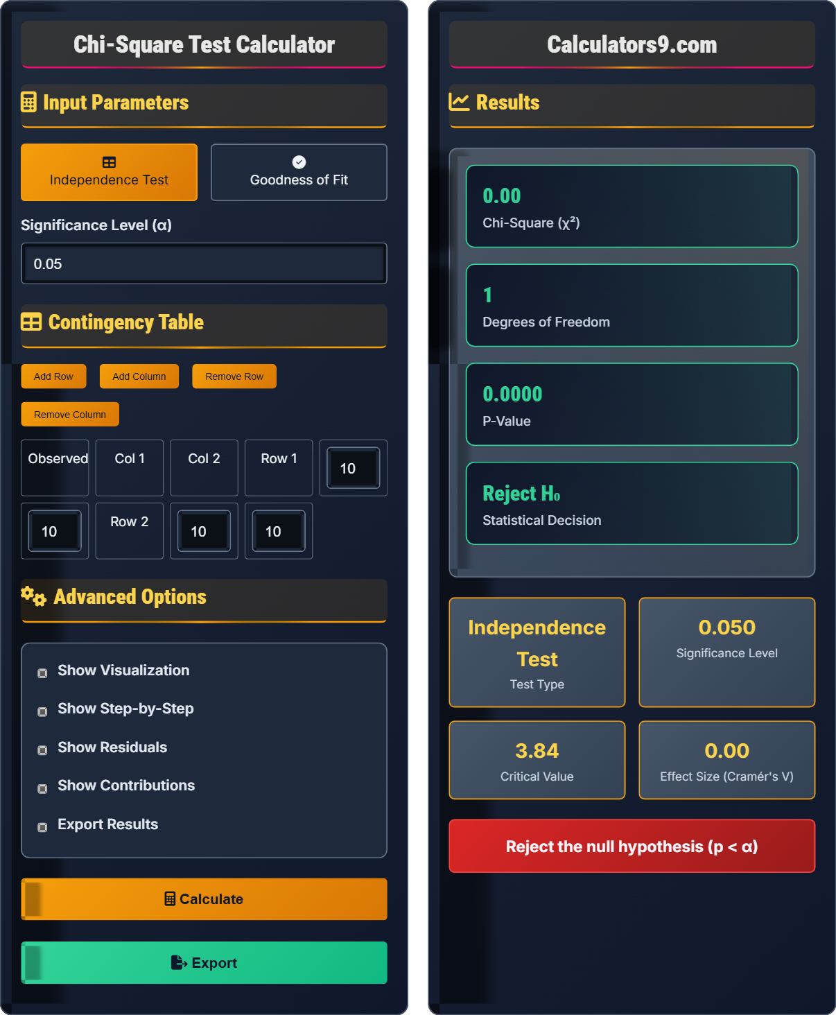
Input Parameters
Independence Test
Goodness of Fit
Contingency Table
Goodness of Fit
Advanced Options
Results
Comprehensive Statistics Guide
The chi-square test is a statistical method used to determine whether there is a significant association between two categorical variables in a contingency table. It compares observed frequencies to expected frequencies under the null hypothesis of independence. The test statistic follows a chi-square distribution and is calculated as the sum of squared differences between observed and expected frequencies, divided by expected frequencies.
The chi-square test statistic is calculated using:
Where:
- \( \chi^2 \) = Chi-square test statistic
- \( O_i \) = Observed frequency in cell i
- \( E_i \) = Expected frequency in cell i
For valid chi-square test results:
- Independence: Observations must be independent
- Expected Frequencies: No more than 20% of cells should have expected frequency < 5
- Sample Size: Generally requires sample size ≥ 50
- Categorical Data: Variables must be categorical
- Large χ² value: Indicates strong evidence against independence
- Small p-value: Suggests significant association between variables
- Effect Size: Use Cramér's V to measure strength of association
- Post-hoc Analysis: Examine standardized residuals to identify specific associations
Statistics Fundamentals
Tests for association between categorical variables using observed vs expected frequencies.
\( \chi^2 = \sum \frac{(O - E)^2}{E} \)
Where χ²=chi-square, O=observed, E=expected frequencies.
- df = (rows-1)(cols-1)
- Expected freq ≥ 5 in most cells
- Independence of observations
Applications
Used in survey analysis, market research, genetics, medical studies, and quality control.
- Set significance level (α)
- Calculate observed and expected frequencies
- Compute chi-square statistic
- Determine degrees of freedom
- Find p-value
- Make statistical decision
- Check expected frequency assumptions
- Consider effect size measures
- Examine residuals for insights
- Sample size affects power
Statistics Learning Quiz
Which of the following statements about chi-square tests is CORRECT?
The answer is B) Chi-square tests are used for categorical variables. Chi-square tests are specifically designed for categorical data analysis. They compare observed frequencies to expected frequencies in contingency tables. The test does not assume normal distribution and cannot be used with continuous variables directly.
This is a fundamental concept in statistics. Chi-square tests are non-parametric tests that work with categorical data. Unlike parametric tests that assume specific distributions, chi-square tests work with frequency counts. The test evaluates whether observed frequencies differ significantly from expected frequencies under the null hypothesis of independence or no association.
Categorical Variable: A variable that can take on one of a limited number of categories
Contingency Table: A table showing the frequency distribution of variables
Non-Parametric Test: A statistical test that doesn't assume a specific distribution
• Chi-square tests require categorical data
• Data must be in frequency format
• Observations must be independent
• Always check expected frequency assumptions
• Use Yates' correction for 2×2 tables
• Consider effect size measures like Cramér's V
• Applying chi-square to continuous data
A researcher collects data on gender (Male/Female) and preference for a product (Yes/No). The observed frequencies are: Male-Yes: 40, Male-No: 60, Female-Yes: 30, Female-No: 70. Calculate the chi-square statistic. Show your work.
First, construct the contingency table with totals:
| Yes | No | Total | |
|---|---|---|---|
| Male | 40 | 60 | 100 |
| Female | 30 | 70 | 100 |
| Total | 70 | 130 | 200 |
Calculate expected frequencies: Eᵢⱼ = (Row Total × Col Total) / Grand Total
E₁₁ = (100 × 70) / 200 = 35
E₁₂ = (100 × 130) / 200 = 65
E₂₁ = (100 × 70) / 200 = 35
E₂₂ = (100 × 130) / 200 = 65
Calculate chi-square: χ² = Σ[(O - E)²/E]
χ² = [(40-35)²/35] + [(60-65)²/65] + [(30-35)²/35] + [(70-65)²/65]
χ² = [25/35] + [25/65] + [25/35] + [25/65] = 0.714 + 0.385 + 0.714 + 0.385 = 2.198
Therefore, χ² ≈ 2.20.
This problem demonstrates the systematic approach to calculating chi-square statistics. First, organize the data in a contingency table with marginal totals. Then calculate expected frequencies under the null hypothesis of independence. Finally, compute the chi-square statistic by summing the squared standardized residuals. Each term (O-E)²/E represents the contribution of that cell to the overall test statistic.
Expected Frequency: Frequency expected under null hypothesis of independence
Marginal Totals: Row and column totals in contingency table
Standardized Residual: (O-E)/√E, measures deviation from independence
• Expected frequency = (row total × col total) / grand total
• df = (rows-1)(cols-1)
• At least 80% of cells should have expected ≥ 5
• Always create a contingency table first
• Double-check your arithmetic
• Verify that row and column totals are consistent
• Incorrectly calculating expected frequencies
• Forgetting to divide by expected frequency
• Not checking assumptions before testing
A study examines the relationship between education level (High School, College, Graduate) and job satisfaction (Satisfied, Neutral, Dissatisfied). The observed frequencies are: [30, 20, 10], [25, 35, 15], [15, 25, 10]. Calculate the chi-square statistic and determine if there is a significant relationship at α = 0.05.
First, organize the data in a contingency table:
| Satisfied | Neutral | Dissatisfied | Total | |
|---|---|---|---|---|
| HS | 30 | 20 | 10 | 60 |
| College | 25 | 35 | 15 | 75 |
| Graduate | 15 | 25 | 10 | 50 |
| Total | 70 | 80 | 35 | 185 |
Calculate expected frequencies: Eᵢⱼ = (Row Total × Col Total) / Grand Total
HS-Satisfied: (60×70)/185 = 22.70
HS-Neutral: (60×80)/185 = 25.95
HS-Dissatisfied: (60×35)/185 = 11.35
College-Satisfied: (75×70)/185 = 28.38
College-Neutral: (75×80)/185 = 32.43
College-Dissatisfied: (75×35)/185 = 14.19
Graduate-Satisfied: (50×70)/185 = 18.92
Graduate-Neutral: (50×80)/185 = 21.62
Graduate-Dissatisfied: (50×35)/185 = 9.46
Calculate chi-square: χ² = Σ[(O - E)²/E] = 4.15
Degrees of freedom: df = (3-1)(3-1) = 4
For α = 0.05 and df = 4, critical value = 9.488
Since 4.15 < 9.488, we fail to reject H₀.
Conclusion: There is no significant relationship between education level and job satisfaction at α = 0.05.
This problem involves a 3×3 contingency table, demonstrating the generalization of the chi-square test. The calculation follows the same principle as the 2×2 case, but with more cells. The degrees of freedom formula (rows-1)(cols-1) works for any size table. The decision rule remains the same: compare the calculated chi-square to the critical value from the chi-square distribution.
Contingency Table: Cross-tabulation of two categorical variables
Degrees of Freedom: Number of values free to vary in chi-square calculation
Independence: No association between categorical variables
• df = (rows-1)(cols-1) for contingency tables
• Always verify expected frequency assumptions
• Check for practical significance beyond statistical significance
• Use technology for larger tables to avoid calculation errors
• Consider standardized residuals to identify specific associations
• Report effect size along with significance
• Incorrectly calculating degrees of freedom
• Not checking expected frequency assumptions
• Misinterpreting non-significant results as evidence of independence
A genetics researcher hypothesizes that a genetic trait follows a 9:3:3:1 ratio (dominant-dominant, dominant-recessive, recessive-dominant, recessive-recessive). In a sample of 200 individuals, the observed frequencies are: 110, 30, 35, 25. Perform a chi-square goodness of fit test at α = 0.05. Does the data support the hypothesis?
Set up hypotheses:
H₀: Trait follows 9:3:3:1 ratio
H₁: Trait does not follow 9:3:3:1 ratio
Calculate expected frequencies based on 9:3:3:1 ratio:
Expected frequencies = [9/16×200, 3/16×200, 3/16×200, 1/16×200] = [112.5, 37.5, 37.5, 12.5]
Calculate chi-square: χ² = Σ[(O - E)²/E]
χ² = [(110-112.5)²/112.5] + [(30-37.5)²/37.5] + [(35-37.5)²/37.5] + [(25-12.5)²/12.5]
χ² = [6.25/112.5] + [56.25/37.5] + [6.25/37.5] + [156.25/12.5]
χ² = 0.056 + 1.5 + 0.167 + 12.5 = 14.223
Degrees of freedom: df = 4 - 1 - 1 = 2 (categories - 1 - parameters estimated)
For α = 0.05 and df = 2, critical value = 5.991
Since 14.223 > 5.991, we reject H₀.
Conclusion: The data does not support the hypothesis of a 9:3:3:1 ratio.
This demonstrates the chi-square goodness of fit test, which compares observed frequencies to expected frequencies based on a theoretical distribution. The degrees of freedom calculation differs from independence tests: df = number of categories - 1 - number of parameters estimated. The test reveals whether the observed data significantly deviates from the expected distribution. The large chi-square value indicates substantial deviation from the expected 9:3:3:1 ratio.
Goodness of Fit Test: Tests whether observed frequencies match expected frequencies
Expected Ratio: Theoretical distribution under null hypothesis
Parameters Estimated: Number of parameters calculated from data
• df = categories - 1 - parameters estimated
• Expected frequency should be ≥ 5 in most cells
• Verify that all observed frequencies are non-negative
• Ensure total observed equals total expected
• Consider biological plausibility of results
• Look for patterns in deviations from expected
• Incorrectly calculating degrees of freedom
• Forgetting to check expected frequency assumptions
• Not accounting for estimated parameters in df calculation
Which of the following is a requirement for valid chi-square test results?
The answer is B) Observations must be independent. Independence of observations is a fundamental requirement for chi-square tests. The test assumes that each observation contributes independently to the frequency count. Chi-square tests do not require normal distribution, work with categorical variables (not interval scale), and generally require larger sample sizes.
Independence is crucial because the chi-square test relies on the assumption that each observation is equally likely to fall into any category based on the underlying probabilities. If observations are dependent (e.g., paired data, clustered data), the test statistic will not follow the chi-square distribution, leading to incorrect conclusions. Other assumptions include having adequate expected frequencies and categorical data.
Independence: One observation does not influence another
Expected Frequency: Frequency expected under null hypothesis
Categorical Data: Data that falls into discrete categories
• Observations must be independent
• Data must be categorical
• Expected frequencies should generally be ≥ 5
• Verify independence before applying the test
• Combine categories if expected frequencies are too low
• Consider Fisher's exact test for small samples
• Applying chi-square to dependent observations
• Ignoring expected frequency assumptions
• Using chi-square for ordinal data without considering order
FAQ
Q: What's the difference between chi-square test of independence and goodness of fit?
A: The chi-square test of independence examines whether two categorical variables are related in a contingency table:
\( H_0: \text{Variables are independent} \)
\( H_1: \text{Variables are associated} \)
The chi-square goodness of fit test compares observed frequencies to expected frequencies for a single categorical variable:
\( H_0: \text{Observed matches expected distribution} \)
\( H_1: \text{Observed does not match expected distribution} \)
For independence: \( df = (r-1)(c-1) \) where r and c are rows and columns
For goodness of fit: \( df = k-1-p \) where k is categories and p is estimated parameters
Q: How do I interpret standardized residuals in chi-square tests?
A: Standardized residuals help identify which cells contribute most to the chi-square statistic:
\( \text{Std Residual} = \frac{O_{ij} - E_{ij}}{\sqrt{E_{ij}}} \)
Interpretation:
- Std residual > 2: More observed than expected
- Std residual < -2: Fewer observed than expected
- |Std residual| > 2: Significant contribution to χ²
These residuals reveal specific patterns of association beyond the overall test result. For example, if studying education and job satisfaction, a large positive residual in the "Graduate-Satisfied" cell would suggest that graduates are more satisfied than expected under independence.