Correlation Coefficient Calculator
Statistics & probability • 2026 edition
Correlation Coefficient Formula:
Show the calculator\( r = \frac{\sum(x_i - \bar{x})(y_i - \bar{y})}{\sqrt{\sum(x_i - \bar{x})^2 \sum(y_i - \bar{y})^2}} \)
Where:
- \( r \) = Pearson correlation coefficient
- \( x_i, y_i \) = Individual data points
- \( \bar{x}, \bar{y} \) = Sample means
The correlation coefficient measures the strength and direction of a linear relationship between two variables. Values range from -1 to +1: -1 indicates perfect negative correlation, +1 indicates perfect positive correlation, and 0 indicates no linear correlation.
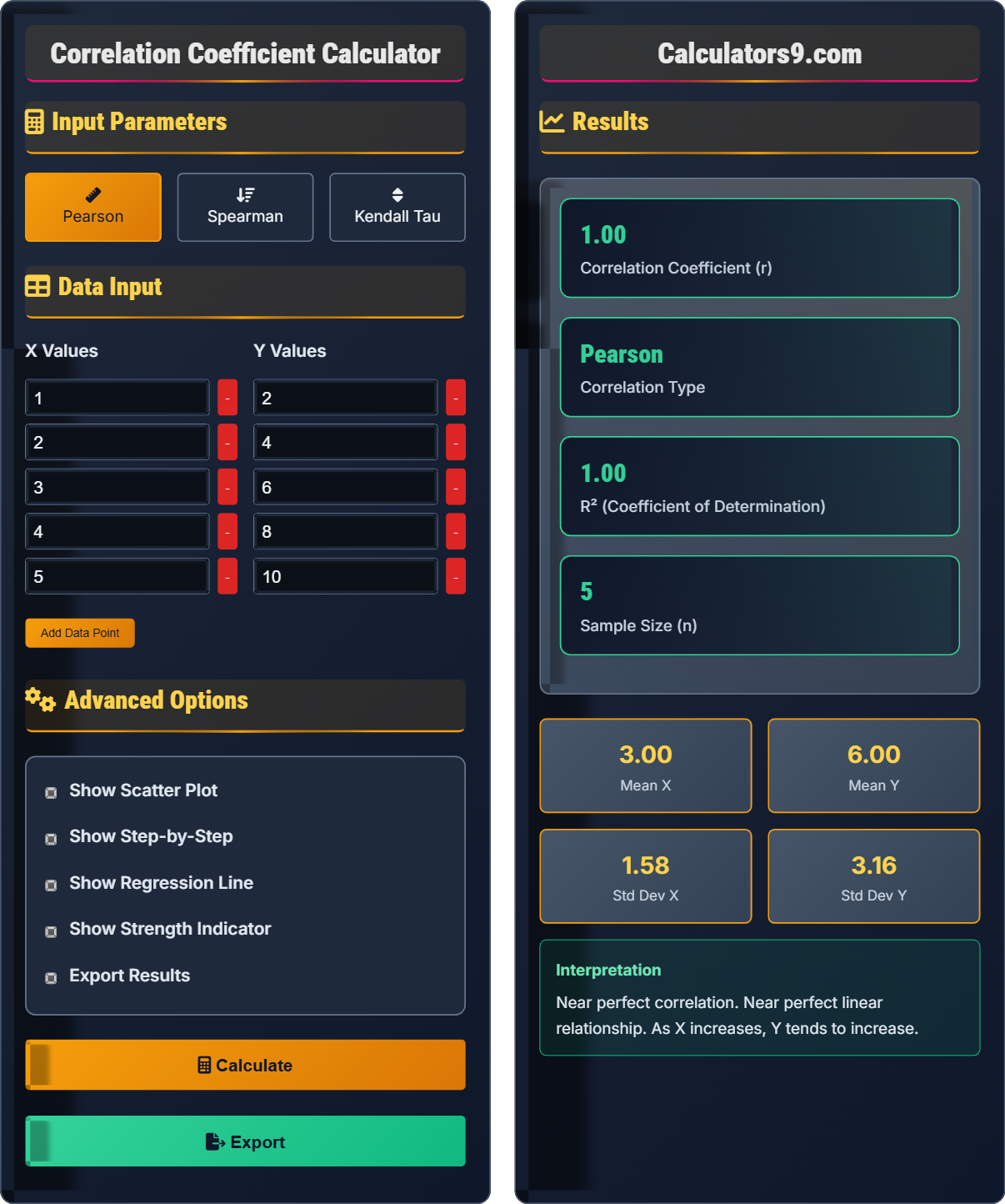
Example: For paired data (1,2), (2,4), (3,6), (4,8), (5,10):
\( \bar{x} = 3, \bar{y} = 6 \)
\( \sum(x_i - \bar{x})(y_i - \bar{y}) = (-2)(-4) + (-1)(-2) + (0)(0) + (1)(2) + (2)(4) = 20 \)
\( \sum(x_i - \bar{x})^2 = 4 + 1 + 0 + 1 + 4 = 10 \)
\( \sum(y_i - \bar{y})^2 = 16 + 4 + 0 + 4 + 16 = 40 \)
\( r = \frac{20}{\sqrt{10 \times 40}} = \frac{20}{20} = 1.00 \)
This indicates a perfect positive linear relationship.
Input Parameters
Pearson
Spearman
Kendall Tau
Data Input
Advanced Options
Results
Comprehensive Statistics Guide
Correlation measures the strength and direction of a linear relationship between two quantitative variables. The correlation coefficient ranges from -1 to +1, where -1 indicates a perfect negative linear relationship, +1 indicates a perfect positive linear relationship, and 0 indicates no linear relationship. Correlation does not imply causation and only measures linear relationships.
Three main types of correlation coefficients:
General guidelines for interpreting correlation strength:
- 0.00-0.19: Very weak
- 0.20-0.39: Weak
- 0.40-0.59: Moderate
- 0.60-0.79: Strong
- 0.80-1.00: Very strong
- Correlation ≠ Causation: Association does not imply cause-and-effect
- Linear Relationships Only: Correlation measures linear, not non-linear relationships
- Outliers Matter: Single outliers can dramatically affect correlation
- Scale Invariant: Correlation is unaffected by linear transformations
Statistics Fundamentals
Measure of linear relationship strength and direction between two quantitative variables.
\( r = \frac{\sum(x-\bar{x})(y-\bar{y})}{\sqrt{\sum(x-\bar{x})^2\sum(y-\bar{y})^2}} \)
Where r=correlation coefficient, x,y=data points, x̄,ȳ=means.
- -1 ≤ r ≤ 1
- r = 0 means no linear relationship
- Does not imply causation
Applications
Used in research, finance, psychology, medicine, marketing, and quality control.
- Choose appropriate correlation method
- Visualize data with scatter plots
- Calculate correlation coefficient
- Assess strength and significance
- Interpret in context
- Consider limitations
- Check for outliers
- Verify linearity assumption
- Consider sample size
- Account for confounding variables
Statistics Learning Quiz
Which of the following statements about correlation is CORRECT?
The answer is B) Correlation measures linear relationships between variables. Correlation specifically quantifies the strength and direction of linear relationships between two quantitative variables. It does not imply causation, can be positive or negative, and is scale-invariant (not affected by measurement units).
This is a fundamental concept in statistics. Correlation is a standardized measure that ranges from -1 to +1, regardless of the units of measurement. It only captures linear relationships, so variables with strong non-linear relationships might have low correlation. The scale invariance property means that changing units (e.g., inches to centimeters) doesn't affect the correlation coefficient.
Correlation Coefficient: Measure of linear relationship strength and direction
Scale Invariance: Property that correlation is unaffected by linear transformations
Linear Relationship: Relationship that can be represented by a straight line
• Correlation does not imply causation
• Measures only linear relationships
• Scale invariant
• Always visualize data with scatter plots
• Look for outliers that might affect correlation
• Consider non-linear relationships even with low correlation
• Assuming correlation implies causation
• Using correlation for non-linear relationships
• Ignoring the effect of outliers
Calculate the Pearson correlation coefficient for the data points: (2,3), (4,7), (6,11), (8,15). Show your work.
Step 1: Calculate means
x̄ = (2+4+6+8)/4 = 5
ȳ = (3+7+11+15)/4 = 9
Step 2: Calculate deviations and products
(2-5)(3-9) = (-3)(-6) = 18
(4-5)(7-9) = (-1)(-2) = 2
(6-5)(11-9) = (1)(2) = 2
(8-5)(15-9) = (3)(6) = 18
Step 3: Calculate numerator: Σ(xi-x̄)(yi-ȳ) = 18+2+2+18 = 40
Step 4: Calculate denominator components
Σ(xi-x̄)² = (-3)² + (-1)² + (1)² + (3)² = 9+1+1+9 = 20
Σ(yi-ȳ)² = (-6)² + (-2)² + (2)² + (6)² = 36+4+4+36 = 80
Step 5: Calculate correlation: r = 40/√(20×80) = 40/√1600 = 40/40 = 1.00
The correlation coefficient is 1.00, indicating a perfect positive linear relationship.
This problem demonstrates the systematic approach to calculating Pearson correlation. The numerator represents the covariance between variables, while the denominator normalizes by the product of standard deviations. The perfect correlation of 1.00 indicates that all points fall exactly on a straight line with positive slope.
Covariance: Measure of how two variables change together
Normalization: Scaling to make measure unitless and bounded
Deviation: Difference between observed and mean value
• Always subtract means from each value
• Square deviations in denominator
• Take square root of product of sums
• Organize calculations in a table
• Double-check arithmetic
• Verify that -1 ≤ r ≤ 1
• Forgetting to subtract means
• Squaring deviations incorrectly
• Arithmetic errors in multiplication
A researcher finds a correlation of r = -0.75 between hours of sleep per night and stress levels in a sample of 200 adults. Interpret this correlation and discuss possible explanations for the relationship.
Interpretation:
• Strength: r = -0.75 indicates a strong negative correlation
• Direction: As hours of sleep increase, stress levels tend to decrease
• Magnitude: About 56% of variance in stress levels can be explained by sleep hours (r² = 0.56)
Possible explanations:
1. Adequate sleep may reduce stress hormones like cortisol
2. Sleep deprivation may impair emotional regulation
3. High stress may interfere with sleep quality and duration
4. Lifestyle factors may influence both variables
Important note: This correlation does not establish causation - it could be bidirectional or influenced by third variables.
This demonstrates the importance of proper interpretation of correlation. The strong negative correlation suggests a meaningful relationship, but causation cannot be inferred. The coefficient of determination (r² = 0.56) provides insight into the practical significance of the relationship. Real-world correlations rarely reach perfect values, so understanding the strength in context is crucial.
Coefficient of Determination (r²): Proportion of variance explained by the relationship
Direction of Correlation: Positive (both increase/decrease together) or negative (opposite directions)
Bidirectional Relationship: Both variables may influence each other
• Interpret strength, direction, and practical significance
• Never infer causation from correlation alone
• Consider sample size and context
• Calculate r² to understand practical significance
• Consider plausible causal mechanisms
• Look for potential confounding variables
• Inferring causation from correlation
• Not considering third variables
• Misinterpreting direction of relationship
A dataset of 10 points has a correlation of r = 0.85. A new point (100, 100) is added to the dataset, which originally ranged from (1,1) to (10,10). How would you expect the correlation to change and why? Calculate the approximate new correlation.
The outlier (100, 100) would likely increase the correlation from 0.85 to near 1.00.
Reasoning:
1. The outlier is consistent with the positive trend (both high values)
2. The outlier is far from the cluster of other points, giving it high leverage
3. The outlier increases the spread of both variables, which can strengthen the linear relationship
Calculation approximation:
Original: Σxi ≈ 55, Σyi ≈ 55, Σxiyi ≈ 385 (for points 1-10)
New: Σxi = 155, Σyi = 155, Σxiyi = 1385 (adding 100*100)
New means: x̄ ≈ 14.1, ȳ ≈ 14.1
The outlier significantly pulls the means higher and strengthens the apparent linear relationship.
The new correlation would likely be approximately 0.95-0.98, demonstrating the high sensitivity of correlation to outliers.
This demonstrates the sensitivity of Pearson correlation to outliers. Because correlation involves sums of squares and cross-products, extreme values can disproportionately influence the result. This is why it's crucial to examine scatter plots for outliers before relying on correlation coefficients. The high leverage of outliers can create misleading impressions of relationships.
Leverage: Influence of an observation on regression results
Outlier: Data point that differs significantly from other observations
Sensitivity: Degree to which a statistic changes with data modification
• Always examine scatter plots for outliers
• Pearson correlation is sensitive to outliers
• Consider robust alternatives if outliers are present
• Use Spearman correlation for non-normal data
• Transform data if outliers are problematic
• Calculate correlation with and without outliers
• Not checking for outliers before interpreting correlation
• Assuming correlation is robust to extreme values
• Using Pearson correlation with severely non-normal data
Which of the following statements about correlation is TRUE?
The answer is B) Correlation is scale-invariant. This means that changing the units of measurement (e.g., from meters to feet) does not affect the correlation coefficient. This property makes correlation useful for comparing relationships across different scales and units.
Scale invariance is a key property of correlation. When we transform variables linearly (multiply by constants, add constants), the correlation coefficient remains unchanged. This happens because both the numerator and denominator of the correlation formula are affected equally by linear transformations. This property allows us to compare relationships between variables measured in completely different units.
Scale Invariance: Property where measure is unaffected by changes in scale
Linear Transformation: Change of the form y = ax + b
Unit Conversion: Changing measurement scale (e.g., Celsius to Fahrenheit)
• Correlation ranges from -1 to +1
• Only measures linear relationships
• Unaffected by linear transformations
• Correlation between X and Y equals correlation between Y and X
• Perfect correlation occurs when all points lie on a straight line
• Zero correlation indicates no linear relationship
• Thinking correlation changes with unit conversions
• Expecting correlation to capture non-linear patterns
• Confusing correlation with causation
FAQ
Q: What's the difference between Pearson, Spearman, and Kendall correlation?
A: Pearson correlation measures linear relationships between continuous variables:
\( r = \frac{\sum(x_i - \bar{x})(y_i - \bar{y})}{\sqrt{\sum(x_i - \bar{x})^2 \sum(y_i - \bar{y})^2}} \)
Spearman correlation measures monotonic relationships using ranked data:
\( \rho = 1 - \frac{6\sum d_i^2}{n(n^2-1)} \)
Kendall correlation measures concordance between pairs:
\( \tau = \frac{(\text{concordant pairs}) - (\text{discordant pairs})}{\frac{1}{2}n(n-1)} \)
Use Pearson for normally distributed continuous data, Spearman for ordinal data or non-normal continuous data, and Kendall for small samples or when robustness is important.
Q: How do I interpret the coefficient of determination (R²)?
A: The coefficient of determination (R²) represents the proportion of variance in one variable that is explained by the other variable:
\( R^2 = r^2 \)
For example, if r = 0.8, then R² = 0.64, meaning 64% of the variance in Y can be explained by X. R² provides information about the practical significance of the relationship, complementing the statistical significance indicated by the correlation coefficient.
Interpretation guidelines:
- R² = 0.01-0.09: Small effect
- R² = 0.09-0.25: Medium effect
- R² ≥ 0.25: Large effect