Exponential Distribution Calculator
Statistics & probability • 2026 edition
Exponential Distribution Formula:
Show the calculator\( f(x) = \lambda e^{-\lambda x} \)
\( F(x) = 1 - e^{-\lambda x} \)
Where:
- \( f(x) \) = Probability density function
- \( F(x) \) = Cumulative distribution function
- \( \lambda \) = Rate parameter (λ > 0)
- \( x \) = Time until event (x ≥ 0)
- \( e \) = Euler's number (~2.718)
The exponential distribution models the time between events in a Poisson process, where events occur continuously and independently at a constant average rate. It's memoryless, meaning the probability of an event occurring in the next time interval doesn't depend on how much time has already passed.
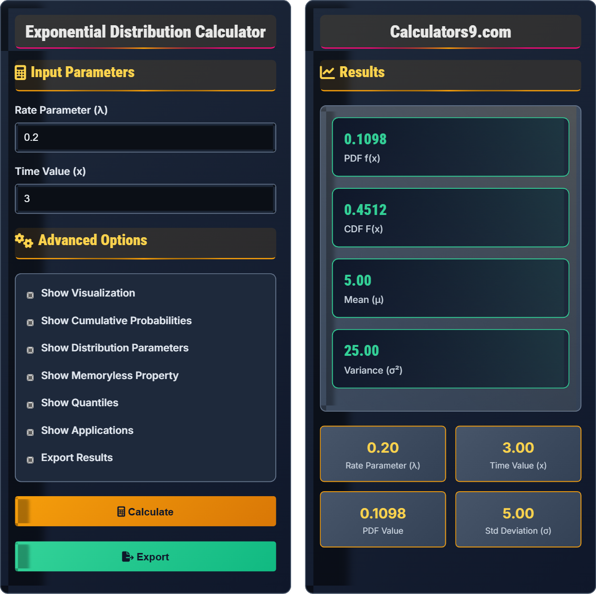
Example: If buses arrive at a stop according to a Poisson process with rate λ = 0.2 per minute (every 5 minutes on average), the probability that the wait time is less than 3 minutes is:
\( F(3) = 1 - e^{-0.2 \times 3} = 1 - e^{-0.6} = 1 - 0.5488 = 0.4512 \)
So there's a 45.12% chance of waiting less than 3 minutes.
Input Parameters
Advanced Options
Results
Comprehensive Statistics Guide
The exponential distribution is a continuous probability distribution that models the time between events in a Poisson process. It's characterized by its memoryless property, meaning the probability of an event occurring in the next time interval is independent of how much time has already passed. This makes it particularly useful for modeling waiting times, lifetimes, and reliability.
Probability density function (PDF):
Cumulative distribution function (CDF):
Key parameters of exponential distribution:
- Mean: μ = 1/λ
- Variance: σ² = 1/λ²
- Standard Deviation: σ = 1/λ
- Median: ln(2)/λ
- Mode: 0
- Skewness: 2
- Queuing Theory: Time between customer arrivals
- Reliability Engineering: Component lifetime
- Telecommunications: Time between phone calls
- Physics: Time until radioactive decay
- Finance: Time until default events
Statistics Fundamentals
Continuous distribution modeling time between events in Poisson process with rate parameter λ.
\( f(x) = \lambda e^{-\lambda x} \)
Where λ=rate parameter, x=time, e=Euler's number.
- x must be non-negative
- λ must be positive
- Memoryless property holds
Applications
Used in queuing theory, reliability analysis, survival analysis, and time-to-event modeling.
- Identify exponential conditions
- Determine rate parameter λ
- Specify time value x
- Apply appropriate formula
- Calculate PDF or CDF
- Interpret results in context
- Verify memoryless assumption
- Check constant rate assumption
- Consider independence of events
- Account for competing risks
Statistics Learning Quiz
Which of the following is a key characteristic of the exponential distribution?
The answer is B) It has the memoryless property. This is the defining characteristic of the exponential distribution. The memoryless property means that the probability of an event occurring in the next time interval is independent of how much time has already passed. This property is unique to the exponential distribution among continuous distributions.
The memoryless property is fundamental to understanding exponential distribution. It means that the distribution "forgets" the past - the probability of waiting an additional time t is the same regardless of how long you've already waited. This makes it ideal for modeling events that occur randomly and independently at a constant rate.
Memoryless Property: P(X > s+t | X > s) = P(X > t)
Continuous Distribution: Defined for all values in an interval
Rate Parameter: Average number of events per unit time
• Memoryless property holds
• Continuous distribution
• Rate parameter λ > 0
• Look for "time until event" problems
• Check for constant rate assumption
• Verify independence of events
• Applying to dependent events
The time between customer arrivals at a store follows an exponential distribution with rate parameter λ = 0.5 per minute. What is the probability that a customer arrives within 2 minutes? Show your work.
Given: λ = 0.5 per minute, need P(X ≤ 2)
Step 1: Apply CDF formula:
\( F(x) = 1 - e^{-\lambda x} \)
Step 2: Substitute values:
\( F(2) = 1 - e^{-0.5 \times 2} = 1 - e^{-1} \)
Step 3: Calculate:
\( F(2) = 1 - 0.3679 = 0.6321 \)
Therefore, there is a 63.21% probability that a customer arrives within 2 minutes.
This problem demonstrates the use of the CDF to find the probability of an event occurring within a certain time. The exponential CDF gives the probability that the waiting time is less than or equal to a specific value. The key is to recognize that P(X ≤ x) is the CDF evaluated at x.
Cumulative Distribution Function: Probability that X ≤ x
Rate Parameter: Average number of events per unit time
Waiting Time: Time until next event occurs
• Use CDF for P(X ≤ x)
• Use 1 - CDF for P(X > x)
• λ must be positive
• Remember: P(X > x) = e^(-λx)
• Use calculator for e^(-λx)
• Check that probability is between 0 and 1
• Using PDF instead of CDF
• Forgetting to subtract from 1
• Incorrectly calculating exponent
A component has an exponential failure distribution with a failure rate of 0.01 failures per hour. What is the probability that the component operates for more than 100 hours? What is the mean time to failure?
Given: λ = 0.01 per hour, need P(X > 100) and mean time to failure
Step 1: Calculate P(X > 100) using the complement of CDF:
\( P(X > 100) = 1 - F(100) = 1 - (1 - e^{-\lambda \times 100}) = e^{-\lambda \times 100} \)
Step 2: Substitute values:
\( P(X > 100) = e^{-0.01 \times 100} = e^{-1} = 0.3679 \)
Step 3: Calculate mean time to failure:
\( \text{MTTF} = \frac{1}{\lambda} = \frac{1}{0.01} = 100 \text{ hours} \)
Therefore, there is a 36.79% probability that the component operates for more than 100 hours, and the mean time to failure is 100 hours.
This problem demonstrates two key applications of the exponential distribution in reliability engineering. The probability that a component survives beyond time t is given by the survival function (complement of CDF). The mean time to failure is simply the reciprocal of the failure rate, which is a special property of the exponential distribution.
Failure Rate: Rate parameter λ in reliability context
Mean Time to Failure: Average time until component fails
Survival Function: P(X > t) = 1 - F(t)
• MTTF = 1/λ
• P(X > t) = e^(-λt)
• Exponential distribution for lifetimes
• Remember: MTTF = 1/λ
• Use survival function for "greater than" problems
• Exponential is common for component lifetimes
• Confusing failure rate with probability
• Using CDF instead of survival function
• Forgetting to take reciprocal for MTTF
Customers arrive at a bank according to a Poisson process with an average of 10 customers per hour. What is the probability that the next customer arrives within 5 minutes? What is the median time between arrivals?
Given: Average arrival rate = 10 per hour, so λ = 10 per hour
Convert 5 minutes to hours: 5/60 = 1/12 hour
Step 1: Calculate P(X ≤ 1/12) using CDF:
\( F(1/12) = 1 - e^{-10 \times (1/12)} = 1 - e^{-10/12} = 1 - e^{-0.8333} \)
Step 2: Calculate:
\( F(1/12) = 1 - 0.4346 = 0.5654 \)
Step 3: Calculate median time between arrivals:
\( \text{Median} = \frac{\ln(2)}{\lambda} = \frac{0.693}{10} = 0.0693 \text{ hours} = 4.16 \text{ minutes} \)
Therefore, there is a 56.54% probability that the next customer arrives within 5 minutes, and the median time between arrivals is 4.16 minutes.
This problem connects the Poisson process (counting events) with the exponential distribution (waiting times). If events follow a Poisson process with rate λ, then the interarrival times follow an exponential distribution with the same rate parameter λ. The median is the value where 50% of the probability lies below it.
Poisson Process: Random process where events occur independently at constant rate
Interarrival Time: Time between consecutive events
Median: Value where 50% of probability is below
• Poisson arrivals → Exponential interarrival times
• Median = ln(2)/λ
• Same λ parameter for both distributions
• Convert time units consistently
• ln(2) ≈ 0.693
• Use 1/λ for mean, ln(2)/λ for median
• Forgetting to convert time units
• Confusing rate parameter with probability
• Using wrong formula for median
Which of the following statements about the memoryless property of the exponential distribution is TRUE?
The answer is B) It only applies to the exponential distribution among continuous distributions. The memoryless property is unique to the exponential distribution in the continuous case. It means that the probability of an event occurring in the next time interval is independent of how much time has already passed. This property makes the exponential distribution particularly useful for modeling events that occur randomly and independently.
The memoryless property is a distinctive characteristic that sets the exponential distribution apart from other continuous distributions. While geometric distribution has a similar property in the discrete case, the exponential distribution is the only continuous distribution with this property. This uniqueness is why the exponential distribution is so important in reliability and queuing theory.
Memoryless Property: P(X > s+t | X > s) = P(X > t)
Continuous Distribution: Distribution defined for continuous values
Uniqueness: Only exponential has this property (continuous)
• Unique to exponential (continuous)
• Geometric has similar property (discrete)
• Independence of past events
• Remember: "No memory" of past events
• Only continuous distribution with this property
• Essential for Markov processes
• Thinking it applies to all distributions
• Confusing with geometric distribution
• Forgetting it's unique to exponential
FAQ
Q: What is the memoryless property and why is it important?
A: The memoryless property states:
\( P(X > s+t | X > s) = P(X > t) \)
This means the probability of waiting an additional time t is the same regardless of how long you've already waited (s). It's important because:
- Models truly random events
- No "aging" effect in reliability
- Simplifies queueing analysis
- Foundational for Markov processes
For example, if a light bulb has exponential lifetime, its probability of lasting another year is the same whether it's brand new or has been operating for 5 years.
Q: How does exponential distribution relate to Poisson distribution?
A: They are complementary distributions:
Poisson: Models number of events in fixed time period
\( P(N = k) = \frac{e^{-\lambda t} (\lambda t)^k}{k!} \)
Exponential: Models time between events
\( f(t) = \lambda e^{-\lambda t} \)
If events follow a Poisson process with rate λ, then the interarrival times follow an exponential distribution with the same rate parameter λ. This relationship is fundamental in queuing theory and reliability analysis.