Normal Distribution CDF Calculator
Statistics & probability • 2026 edition
Normal Distribution CDF Formula:
Show the calculator\( \Phi(x) = \frac{1}{\sqrt{2\pi}} \int_{-\infty}^{x} e^{-\frac{t^2}{2}} dt \)
Where:
- \( \Phi(x) \) = Cumulative distribution function
- \( x \) = Value on the horizontal axis
- \( \mu \) = Mean of the distribution
- \( \sigma \) = Standard deviation
The normal distribution CDF gives the probability that a normally distributed random variable is less than or equal to a specific value. For the standard normal distribution (μ=0, σ=1), the CDF represents the area under the bell curve to the left of a given z-score.
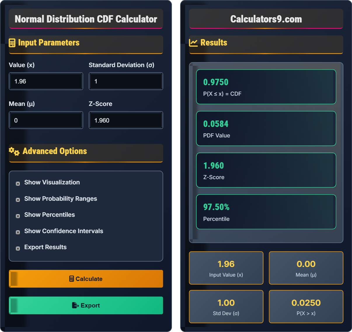
Example: For x=1.96 in standard normal distribution:
\( \Phi(1.96) \approx 0.975 \)
This means P(X ≤ 1.96) = 0.975 or 97.5% of values are below 1.96.
Input Parameters
Advanced Options
Results
Comprehensive Statistics Guide
The cumulative distribution function (CDF) of the normal distribution gives the probability that a normally distributed random variable is less than or equal to a specific value. It represents the area under the normal curve to the left of that value. The CDF is fundamental in statistics for calculating probabilities and percentiles.
The standard normal CDF:
For any normal distribution with mean μ and standard deviation σ:
Special case with μ=0 and σ=1:
- Z-Score: Standardized value: z = (x-μ)/σ
- Common Values: Φ(0) = 0.5, Φ(1) ≈ 0.841, Φ(1.96) ≈ 0.975
- Universal Reference: All normal distributions can be standardized
- Quality Control: Monitoring manufacturing processes
- Finance: Risk modeling and portfolio analysis
- Medicine: Analyzing patient data and test results
- Education: Standardized testing and grading
- Psychology: Intelligence testing and behavioral studies
Statistics Fundamentals
Cumulative distribution function giving probability that normally distributed variable ≤ x.
\( F(x) = \Phi\left(\frac{x-\mu}{\sigma}\right) \)
Where Φ = standard normal CDF, μ = mean, σ = standard deviation.
- Range: 0 ≤ F(x) ≤ 1
- F(∞) = 1, F(-∞) = 0
- F(x) is always increasing
Applications
Used in hypothesis testing, confidence intervals, quality control, and probability calculations.
- Identify mean and standard deviation
- Standardize using z-score formula
- Look up CDF value in table or calculate
- Interpret probability result
- Make statistical decision
- Verify normality assumption
- Consider sample size
- Account for outliers
- Use appropriate distribution
Statistics Learning Quiz
Which of the following statements about the normal distribution is CORRECT?
The answer is B) The normal distribution is symmetric around its mean. The normal distribution is perfectly symmetric around its mean, which is also its median and mode. This is a defining characteristic of the normal distribution.
This is a fundamental property of the normal distribution. The bell-shaped curve is symmetric, meaning that 50% of the values lie below the mean and 50% lie above the mean. The tails of the distribution extend infinitely in both directions but approach zero asymptotically.
Normal Distribution: Continuous probability distribution with bell-shaped curve
Symmetry: Distribution is identical on both sides of the mean
Asymptotic: Approaching but never reaching zero
• Symmetric around mean
• Mean = Median = Mode
• Tails approach zero asymptotically
• Remember the bell shape
• Use symmetry for calculations
• Know the 68-95-99.7 rule
• Thinking it's bounded
• Confusing with other distributions
• Forgetting about symmetry
For a normal distribution with mean μ = 100 and standard deviation σ = 15, find P(X ≤ 115). Show your work.
Step 1: Calculate the z-score:
z = (x - μ) / σ = (115 - 100) / 15 = 15 / 15 = 1.0
Step 2: Find P(Z ≤ 1.0) using standard normal table:
P(Z ≤ 1.0) ≈ 0.8413
Therefore, P(X ≤ 115) = 0.8413 or approximately 84.13%.
This problem demonstrates the standardization process. We convert any normal distribution to the standard normal distribution using the z-score formula. This allows us to use standard normal tables to find probabilities for any normal distribution regardless of its mean and standard deviation.
Z-Score: Standardized value measuring standard deviations from mean
Standardization: Converting to standard normal distributionStandard Normal: Normal distribution with μ=0, σ=1
• z = (x - μ) / σ
• Always standardize first
• Use standard normal tables
• Draw the distribution to visualize
• Check if answer makes sense
• Use technology for precise values
• Forgetting to standardize
• Using wrong formula for z-score
• Looking up wrong value in table
The weight of manufactured widgets follows a normal distribution with mean 50 grams and standard deviation 2 grams. What percentage of widgets weigh between 46 and 54 grams? What is the significance of this range?
Step 1: Calculate z-scores for both values:
For x = 46: z₁ = (46 - 50) / 2 = -4 / 2 = -2.0
For x = 54: z₂ = (54 - 50) / 2 = 4 / 2 = 2.0
Step 2: Find probabilities:
P(Z ≤ -2.0) ≈ 0.0228
P(Z ≤ 2.0) ≈ 0.9772
Step 3: Calculate P(-2.0 ≤ Z ≤ 2.0):
P(-2.0 ≤ Z ≤ 2.0) = P(Z ≤ 2.0) - P(Z ≤ -2.0) = 0.9772 - 0.0228 = 0.9544
Therefore, approximately 95.44% of widgets weigh between 46 and 54 grams.
This range represents the middle 95.44% of the distribution, which is close to the 95% of the 68-95-99.7 rule for values within 2 standard deviations of the mean.
This problem demonstrates finding probabilities for ranges in a normal distribution. We standardize both endpoints and find the difference in their cumulative probabilities. The range from 46 to 54 grams represents values within 2 standard deviations of the mean, which aligns with the empirical rule.
Empirical Rule: 68-95-99.7 rule for normal distribution
Quality Control: Statistical methods to maintain product quality
Acceptable Range: Range of acceptable values
• Standardize both endpoints
• P(a ≤ X ≤ b) = P(X ≤ b) - P(X ≤ a)
• Use symmetry when applicable
• Remember the 68-95-99.7 rule
• Draw the distribution to visualize
• Use complement for easier calculations
• Adding instead of subtracting probabilities
• Forgetting to standardize both values
• Misinterpreting the result
Test scores are normally distributed with mean 75 and standard deviation 10. If a student scores 85, what percentile rank does this correspond to? What percentage of students scored higher than this student?
Step 1: Calculate the z-score:
z = (85 - 75) / 10 = 10 / 10 = 1.0
Step 2: Find P(Z ≤ 1.0) using standard normal table:
P(Z ≤ 1.0) ≈ 0.8413
Step 3: Interpret the results:
The percentile rank is approximately 84.13%, meaning the student scored better than about 84.13% of all students.
The percentage of students who scored higher is:
P(Z > 1.0) = 1 - P(Z ≤ 1.0) = 1 - 0.8413 = 0.1587 or about 15.87%
Therefore, about 15.87% of students scored higher than this student.
This problem demonstrates how to find percentile ranks using the normal distribution. The percentile rank corresponds to the cumulative probability up to that score. The complement gives the percentage scoring higher. This is commonly used in educational and psychological testing.
Percentile Rank: Percentage of scores below a given score
Standard Score: Z-score indicating position relative to mean
Norm-Referenced: Scores compared to group distribution
• Percentile = CDF value × 100
• P(higher) = 1 - P(lower)
• Standardize before looking up
• Use complement for "greater than" questions
• Remember that percentile is cumulative probability
• Draw the distribution to visualize
• Confusing percentile with percentage
• Forgetting to standardize
• Misinterpreting the result
According to the 68-95-99.7 rule, what percentage of data in a normal distribution falls within 1.5 standard deviations of the mean?
The answer is B) 87%. The 68-95-99.7 rule states that approximately 68% of data falls within 1 standard deviation, 95% within 2 standard deviations, and 99.7% within 3 standard deviations. For 1.5 standard deviations, we interpolate between 68% and 95%, which is approximately 87%.
The 68-95-99.7 rule is a useful approximation for normal distributions. For values not exactly matching 1, 2, or 3 standard deviations, we can interpolate or use the standard normal table for precise values. The actual value for 1.5 standard deviations is approximately 86.64%.
Empirical Rule: 68-95-99.7 rule for normal distribution
Standard Deviations: Units measuring distance from mean
Approximation: Close but not exact values
• 1σ: ~68% of data
• 2σ: ~95% of data
• 3σ: ~99.7% of data
• Remember the 68-95-99.7 pattern
• Use interpolation for intermediate values
• For precise values, use standard normal table
• Confusing the percentages
• Not interpolating for intermediate values
• Forgetting that it's an approximation
FAQ
Q: What's the difference between PDF and CDF in normal distribution?
A: The Probability Density Function (PDF) and Cumulative Distribution Function (CDF) are related but different:
PDF: \( f(x) = \frac{1}{\sqrt{2\pi\sigma^2}} e^{-\frac{(x-\mu)^2}{2\sigma^2}} \)
• Gives the density at a specific point (not probability!)
• Forms the bell-shaped curve
• Area under curve between two points gives probability
CDF: \( F(x) = P(X \leq x) = \int_{-\infty}^{x} f(t) dt \)
• Gives the actual probability that X ≤ x
• Always increases from 0 to 1
• The derivative of CDF is PDF
• The integral of PDF is CDF
Q: How do I calculate P(a < X < b) using the normal distribution?
A: To calculate P(a < X < b) for a normal distribution:
1. Standardize both values: \( z_a = \frac{a-\mu}{\sigma} \), \( z_b = \frac{b-\mu}{\sigma} \)
2. Find the CDF values: \( \Phi(z_a) \) and \( \Phi(z_b) \)
3. Calculate: \( P(a < X < b) = \Phi(z_b) - \Phi(z_a) \)
For example, if X ~ N(50, 10²) and we want P(40 < X < 60):
\( z_1 = \frac{40-50}{10} = -1 \), \( z_2 = \frac{60-50}{10} = 1 \)
\( P(40 < X < 60) = \Phi(1) - \Phi(-1) = 0.8413 - 0.1587 = 0.6826 \)