Poisson Distribution Calculator
Statistics & probability • 2026 edition
Poisson Distribution Formula:
Show the calculator\( P(X = k) = \frac{e^{-\lambda} \lambda^k}{k!} \)
Where:
- \( P(X = k) \) = Probability of exactly k events
- \( \lambda \) = Average rate of occurrence (λ > 0)
- \( k \) = Number of events (k ≥ 0)
- \( e \) = Euler's number (~2.718)
The Poisson distribution models the number of events occurring in a fixed interval of time or space, given a known average rate of occurrence. It's used for rare events, counting processes, and modeling arrivals. The distribution assumes events occur independently at a constant average rate.
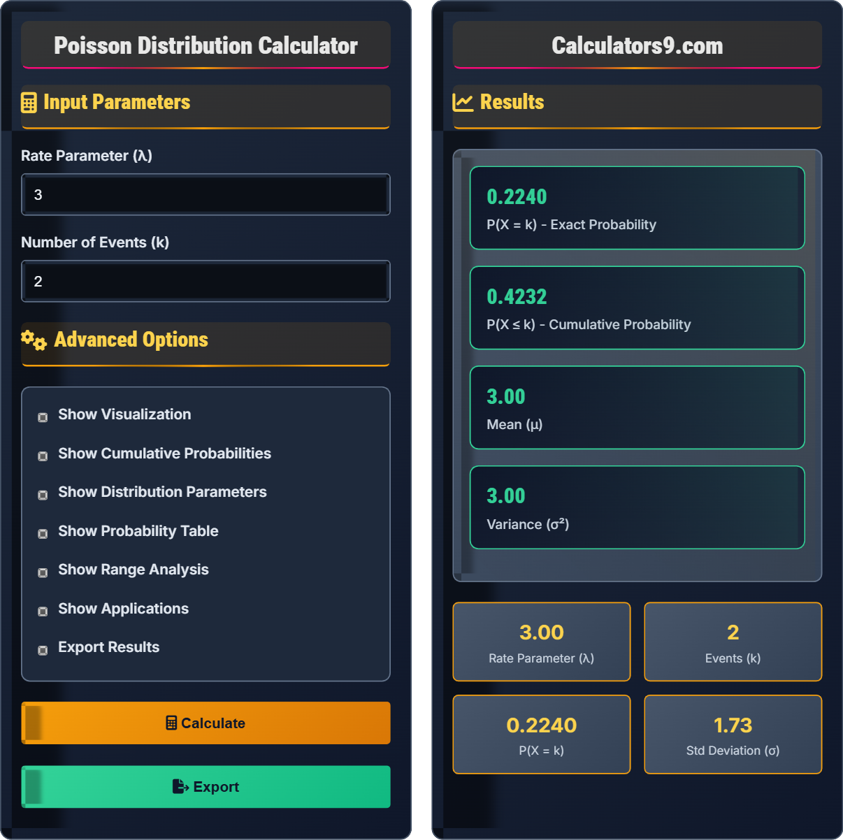
Example: If a call center receives an average of 3 calls per minute (λ = 3), the probability of receiving exactly 2 calls in a minute is:
\( P(X = 2) = \frac{e^{-3} \times 3^2}{2!} = \frac{0.0498 \times 9}{2} = 0.2240 \)
So there's a 22.40% chance of receiving exactly 2 calls in a minute.
Input Parameters
Advanced Options
Results
Comprehensive Statistics Guide
The Poisson distribution is a discrete probability distribution that models the number of events occurring in a fixed interval of time or space, given a known average rate of occurrence. Named after French mathematician Siméon Denis Poisson, it's particularly useful for modeling rare events and counting processes where events occur independently at a constant average rate.
The probability mass function:
Where the cumulative distribution function is:
Key parameters of Poisson distribution:
- Mean: μ = λ
- Variance: σ² = λ
- Standard Deviation: σ = √λ
- Skewness: γ₁ = 1/√λ
- Mode: ⌊λ⌋ (when not integer) or both ⌊λ⌋ and ⌊λ⌋-1
- Call Centers: Phone calls received per hour
- Quality Control: Defects per unit of product
- Transportation: Accidents per day/month
- Healthcare: Patient arrivals per hour
- Physics: Radioactive decay events
Statistics Fundamentals
Discrete distribution modeling rare events in fixed time/space intervals with rate parameter λ.
\( P(X = k) = \frac{e^{-\lambda} \lambda^k}{k!} \)
Where λ=rate parameter, k=number of events, e=Euler's number.
- k must be non-negative integer
- λ must be positive
- Events must occur independently
Applications
Used in telecommunications, quality control, healthcare, physics, and traffic engineering.
- Identify Poisson conditions
- Determine rate parameter λ
- Specify number of events k
- Apply appropriate formula
- Calculate exact or cumulative probability
- Interpret results in context
- Check independence assumption
- Verify constant rate assumption
- Consider sample size limitations
- Account for overdispersion
Statistics Learning Quiz
Which of the following scenarios is best modeled using a Poisson distribution?
The answer is B) Number of accidents at an intersection per month. This scenario fits the Poisson model: it counts discrete events (accidents) occurring in a fixed time interval (month) with a relatively low rate of occurrence. The events are typically independent and occur at a constant average rate.
For Poisson distribution, events must be discrete counts in a fixed interval, occur independently, and have a constant average rate. Rolling dice follows a binomial distribution, tree heights are continuous (normal distribution), and waiting times follow an exponential distribution.
Poisson Distribution: Discrete distribution for rare events in fixed intervals
Rate Parameter: Average number of events per interval (λ)
Discrete Events: Countable occurrences
• Must be discrete counts
• Events must be rare
• Must occur in fixed intervals
• Look for "number of events in interval"
• Check for rare occurrences
• Verify independence of events
• Applying to continuous data
• Using for non-independent events
• Forgetting to verify rate assumptions
A hospital emergency room averages 5 patients per hour. What is the probability that exactly 3 patients arrive in a given hour? Show your work.
Given: λ = 5 (average patients per hour), k = 3 (patients to find probability for)
Step 1: Apply Poisson formula:
\( P(X = 3) = \frac{e^{-\lambda} \lambda^k}{k!} = \frac{e^{-5} \times 5^3}{3!} \)
Step 2: Calculate components:
\( e^{-5} = 0.006738 \)
\( 5^3 = 125 \)
\( 3! = 6 \)
Step 3: Complete calculation:
\( P(X = 3) = \frac{0.006738 \times 125}{6} = \frac{0.84225}{6} = 0.1404 \)
Therefore, there is a 14.04% probability that exactly 3 patients arrive in a given hour.
This problem demonstrates the systematic approach to Poisson calculations. First identify λ (the rate parameter) and k (the specific number of events). Then substitute into the formula, calculating each component separately before combining them. The exponential term represents the decay factor.
Rate Parameter: Average number of events per interval (λ)
Exact Probability: Probability of exactly k events
Factorial: k! = k × (k-1) × ... × 2 × 1
• λ must be positive
• k must be non-negative integer
• Use calculator for complex calculations
• Use scientific calculator for e^(-λ)
• Remember: 0! = 1
• Check that probability is between 0 and 1
• Incorrectly calculating factorial
• Using wrong value for λ
• Forgetting to divide by k!
A manufacturing process produces an average of 0.2 defects per unit. If 100 units are inspected, what is the probability that at most 1 defect is found? What is the expected number of defects?
Given: λ = 0.2 per unit, n = 100 units, so total λ = 0.2 × 100 = 20
Step 1: Calculate P(X ≤ 1) = P(X = 0) + P(X = 1)
For P(X = 0):
\( P(X = 0) = \frac{e^{-20} \times 20^0}{0!} = \frac{e^{-20} \times 1}{1} = e^{-20} \approx 2.06 \times 10^{-9} \)
For P(X = 1):
\( P(X = 1) = \frac{e^{-20} \times 20^1}{1!} = 20 \times e^{-20} \approx 4.12 \times 10^{-8} \)
Step 2: Sum the probabilities:
\( P(X ≤ 1) = 2.06 \times 10^{-9} + 4.12 \times 10^{-8} = 4.33 \times 10^{-8} \)
Step 3: Calculate expected number of defects:
Mean = λ = 20
Therefore, there is virtually zero probability (4.33 × 10⁻⁸) of finding at most 1 defect, and the expected number of defects is 20.
This problem demonstrates scaling the rate parameter when dealing with multiple intervals. Since we're inspecting 100 units, the total expected defects is 100 × 0.2 = 20. With such a high expected value, the probability of finding very few defects is extremely small, which aligns with our intuition.
Cumulative Probability: Probability of at most k events
Expected Value: Long-run average number of events
Quality Control: Statistical methods for monitoring processes
• Scale λ for multiple intervals
• P(X ≤ k) = sum of P(X = i) for i = 0 to k
• Mean = λ for Poisson distribution
• When λ is large, consider normal approximation
• Remember mean = variance in Poisson
• Check for computational feasibility
• Forgetting to scale λ for multiple intervals
• Not handling very small probabilities correctly
• Misinterpreting the result for large λ
A call center receives an average of 8 calls per minute. What is the probability that more than 10 calls arrive in a given minute? What is the probability that between 5 and 12 calls (inclusive) arrive in a minute?
Given: λ = 8, need P(X > 10) and P(5 ≤ X ≤ 12)
Part A: P(X > 10) = 1 - P(X ≤ 10)
Calculating P(X ≤ 10) requires summing P(X = 0) through P(X = 10):
P(X ≤ 10) ≈ 0.8159 (calculated using cumulative Poisson formula)
Therefore: P(X > 10) = 1 - 0.8159 = 0.1841
Part B: P(5 ≤ X ≤ 12) = P(X ≤ 12) - P(X ≤ 4)
Using cumulative probabilities:
P(X ≤ 12) ≈ 0.9362
P(X ≤ 4) ≈ 0.0996
Therefore: P(5 ≤ X ≤ 12) = 0.9362 - 0.0996 = 0.8366
So there is an 18.41% probability of more than 10 calls, and an 83.66% probability of between 5 and 12 calls.
This problem demonstrates calculating probabilities for ranges. For "more than 10", we use the complement: 1 - P(X ≤ 10). For "between 5 and 12", we use: P(X ≤ 12) - P(X ≤ 4). This approach is more efficient than summing individual probabilities for each value in the range.
Range Probability: Probability of event count within a range
Cumulative Approach: Using CDF to find range probabilities
Complement Rule: P(A) = 1 - P(A^c)
• P(a ≤ X ≤ b) = P(X ≤ b) - P(X ≤ a-1)
• P(X > k) = 1 - P(X ≤ k)
• P(X ≥ k) = 1 - P(X ≤ k-1)
• Use complement for "greater than" problems
• Use cumulative approach for ranges
• Consider normal approximation for large λ
• Forgetting to subtract P(X ≤ a-1) for ranges
• Miscounting the number of terms to sum
• Not considering the complement approach
For a Poisson distribution with λ = 4, which of the following statements is TRUE?
The answer is C) Mean = 4. For a Poisson distribution, both the mean and variance equal λ. So with λ = 4, the mean is 4 and the variance is 4. The standard deviation is √λ = √4 = 2.
This question tests the fundamental property of the Poisson distribution: both mean and variance equal the rate parameter λ. This is a unique characteristic that distinguishes the Poisson from other distributions. The standard deviation is always √λ.
Mean: Expected value of the distribution
Variance: Measure of spread around the mean
Standard Deviation: Square root of variance
• Mean = λ
• Variance = λ
• Std Dev = √λ
• Remember mean = variance in Poisson
• Standard deviation is always smaller than mean
• As λ increases, distribution becomes more normal
• Confusing mean and variance values
• Forgetting that mean = variance
• Using wrong formula for standard deviation
FAQ
Q: When should I use Poisson distribution vs Binomial distribution?
A: Use Poisson when:
- Counting events in a fixed interval
- Events occur independently
- Rate parameter λ is known
- Events are rare (n large, p small)
Use Binomial when:
- Fixed number of trials n
- Each trial has binary outcome
- Constant probability p
- Finite number of possible outcomes
The Poisson is the limiting case of Binomial when n → ∞ and p → 0 with np = λ.
Q: What is the relationship between Poisson and Exponential distributions?
A: They are complementary distributions:
Poisson: Models number of events in fixed time period
\( P(X = k) = \frac{e^{-\lambda} \lambda^k}{k!} \)
Exponential: Models time between events
\( f(t) = \lambda e^{-\lambda t} \)
If events follow a Poisson process with rate λ, then the interarrival times follow an exponential distribution with the same rate parameter λ. This relationship is fundamental in queuing theory and reliability analysis.