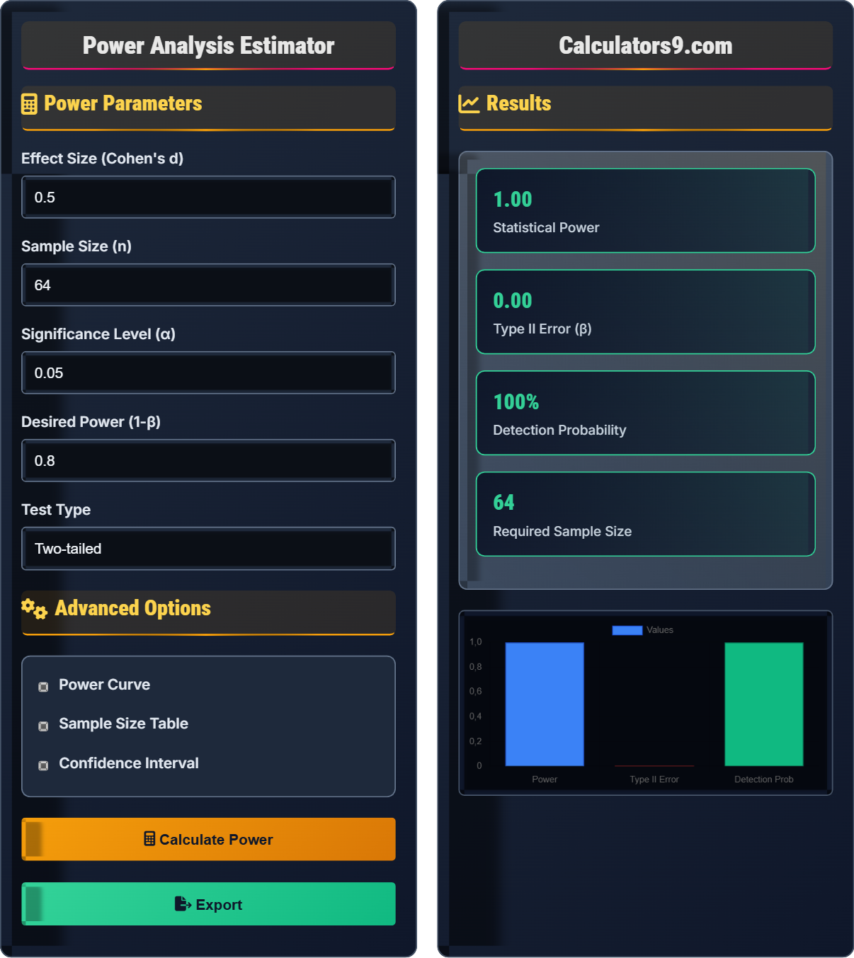
Power Analysis Estimator
Statistical power calculator • Research methodology
Power Analysis Formula:
Show the calculator\( \text{Power} = 1 - \beta \)
Where:
- \( \beta \) = Type II error rate (probability of failing to reject false null hypothesis)
- \( \alpha \) = Significance level (Type I error rate)
- \( d \) = Effect size (Cohen's d)
- \( n \) = Sample size
Power analysis helps determine the probability of detecting an effect if it exists. It balances four key parameters: statistical power, significance level, effect size, and sample size.
Cohen's Effect Size Interpretation:
- Small: d = 0.2
- Medium: d = 0.5
- Large: d = 0.8
For example, with α = 0.05, d = 0.5 (medium effect), n = 64, the power would be approximately 80%.
Power Parameters
Advanced Options
Results
Comprehensive Power Analysis Guide
Power analysis is a statistical technique used to determine the probability that a study will detect an effect if there is one. It helps researchers plan studies by calculating the minimum sample size needed to achieve a desired level of statistical power, ensuring that the study has a good chance of detecting meaningful effects.
The fundamental relationship in power analysis involves four key parameters:
Where:
- \(H_0\): Null hypothesis
- \(H_1\): Alternative hypothesis
- \(\beta\): Probability of Type II error
- \(\alpha\): Significance level (Type I error rate)
Cohen provided conventional benchmarks for interpreting effect sizes:
- Small: d = 0.2 (small but noticeable effect)
- Medium: d = 0.5 (moderate effect)
- Large: d = 0.8 (large and obvious effect)
- A Priori Analysis: Calculating required sample size given power, effect size, and significance level
- Post Hoc Analysis: Calculating achieved power given sample size, effect size, and significance level
- Criterion Analysis: Determining significance level given power, effect size, and sample size
- Two-tailed vs One-tailed: Adjusting for directional hypotheses
Power Analysis Fundamentals
Probability of correctly rejecting a false null hypothesis.
\( \text{Power} = 1 - \beta \)
Where β is the Type II error rate.
- Power increases with larger sample sizes
- Power increases with larger effect sizes
- Power decreases with stricter significance levels
- Standard power threshold is 0.8 (80%)
Research Planning
Measures the magnitude of the phenomenon being studied.
- Determine desired power (usually 0.8)
- Estimate expected effect size
- Set significance level (usually 0.05)
- Calculate required sample size
- Practical significance vs statistical significance
- Resource constraints
- Expected dropout rates
- Multiple comparisons adjustments
Power Analysis Learning Quiz
What does statistical power represent in a research study?
The answer is B) Probability of correctly rejecting a false null hypothesis. Statistical power is defined as the probability of correctly rejecting a false null hypothesis, which means detecting an effect when there actually is one. This is calculated as 1 - β, where β is the probability of a Type II error (failing to reject a false null hypothesis).
Understanding statistical power is crucial for researchers because it tells us the likelihood of finding a significant result when there truly is an effect in the population. A study with low power has a high risk of missing real effects, leading to potentially important findings going undetected. The higher the power, the more confident we can be that non-significant results indicate a true absence of effect rather than just insufficient sample size.
Statistical Power: Probability of correctly rejecting a false null hypothesis (1 - β)
Type I Error (α): Rejecting a true null hypothesis (false positive)
Type II Error (β): Failing to reject a false null hypothesis (false negative)
• Power = 1 - β (probability of avoiding Type II error)
• Standard power threshold is 0.8 (80%)
• Power is about detecting true effects, not avoiding false positives
• Remember: Power = "Power to detect"
• High power means low chance of missing real effects
• Power is about sensitivity to true effects
• Confusing power with significance level (α)
• Thinking power relates to Type I errors
• Misunderstanding that power is about detecting true effects
If a researcher calculates Cohen's d = 0.6, how would you classify this effect size and what does it mean in practical terms?
An effect size of d = 0.6 represents a medium-to-large effect according to Cohen's conventions. Cohen's benchmarks are: Small = 0.2, Medium = 0.5, Large = 0.8. An effect size of 0.6 indicates that the difference between groups is 0.6 standard deviations, which is considered a practically meaningful difference that would be noticeable in real-world applications.
Effect size is crucial because it tells us about the practical significance of a finding, independent of sample size. While statistical significance tells us whether an effect exists, effect size tells us about the magnitude of that effect. A statistically significant result with a small effect size might not be practically meaningful, while a large effect size indicates a substantial difference that matters in practice. Effect size allows for comparison across studies regardless of sample size.
Cohen's d: Standardized measure of effect size for mean differences
Effect Size: Quantitative measure of the magnitude of a phenomenon
Practical Significance: Meaningfulness of an effect in real-world context
• Effect size is independent of sample size
• Cohen's benchmarks: Small (0.2), Medium (0.5), Large (0.8)
• Effect size indicates practical significance
• Remember Cohen's benchmark: 0.2, 0.5, 0.8
• Effect size = mean difference / pooled standard deviation
• Larger effect sizes require smaller samples for same power
• Confusing statistical significance with practical significance
• Ignoring effect size in favor of p-values only
• Misapplying Cohen's benchmarks to all contexts
A researcher wants to conduct a study with 80% power (0.8) to detect a medium effect size (d = 0.5) at a significance level of α = 0.05 for a two-tailed test. Using power analysis, approximately how many participants per group would be needed?
For a two-sample t-test with these parameters:
- Power = 0.8
- Effect size (d) = 0.5
- Significance level (α) = 0.05
- Two-tailed test
This example demonstrates the practical application of power analysis in research planning. The sample size calculation balances four factors: desired power (how confident we want to be in detecting true effects), expected effect size (how large an effect we expect to find), significance level (our threshold for statistical significance), and the type of test (one-tailed vs two-tailed). Researchers must consider these trade-offs when designing studies to ensure adequate statistical power while remaining feasible.
A Priori Power Analysis: Calculating sample size before conducting study
Two-tailed Test: Testing for effects in both directions
Sample Size Calculation: Determining n needed for desired power
• Higher power requires larger sample sizes
• Use software like G*Power for exact calculations
• Plan for potential dropouts (add 10-20% to sample size)
• Consider feasibility when setting power targets
• Using post-hoc power analysis to interpret non-significant results
• Underestimating required sample sizes
• Not accounting for multiple comparisons
A researcher has a fixed budget that allows for either 40 participants with high measurement precision or 80 participants with moderate measurement precision. The expected effect size is medium (d = 0.5). Which option would provide greater statistical power and why? Assume significance level remains at α = 0.05.
The option with 80 participants would provide greater statistical power. Power increases with sample size, and the increase in sample size from 40 to 80 participants would more than compensate for the moderate measurement precision. With n = 40, power would be approximately 0.69, while with n = 80, power would be approximately 0.89 for a medium effect size. The larger sample size provides more statistical power despite the less precise measurements.
This question highlights the fundamental trade-off in research design between sample size and measurement precision. While high precision measurements are valuable, the law of large numbers often makes larger samples more beneficial for statistical power. The relationship between sample size and power follows a square root function, meaning that doubling the sample size increases power significantly. However, this trade-off depends on the cost differential between recruiting additional participants versus improving measurement precision.
Measurement Precision: Accuracy and reliability of measures
Sample Size vs Precision Trade-off: Balance between n and measurement quality
Statistical Efficiency: Achieving goals with minimal resources
• Power increases with sample size
• Larger samples often compensate for imperfect measures
• Consider resource allocation for optimal design
• Calculate power for different scenarios
• Consider cost per participant vs cost per measurement
• Balance power with practical constraints
• Assuming perfect measurements always outweigh sample size
• Not considering the diminishing returns of precision improvements
• Ignoring the statistical impact of sample size increases
Which of the following combinations would result in the highest statistical power?
The answer is B) α = 0.05, d = 0.8, n = 100. This combination has the highest power because it includes a large effect size (d = 0.8), which dramatically increases power, along with a reasonable sample size (n = 100) and standard significance level (α = 0.05). Large effect sizes require smaller samples to achieve the same power, and the combination of large effect size and adequate sample size results in the highest statistical power.
This question demonstrates how the four parameters of power interact. While increasing sample size (option D) might seem to provide the highest power, the extremely strict significance level (α = 0.001) counteracts this advantage. Similarly, option A has a reasonable sample size but suffers from both a very strict significance level and a small effect size. Option B optimally balances all three parameters that enhance power: moderate significance level, large effect size, and adequate sample size.
Power Parameters: α, d, n, and test type
Parameter Interactions: How factors influence each other
Optimal Design: Balancing all parameters effectively
• Power increases with larger effect sizes
• Power increases with larger sample sizes
• Power decreases with stricter significance levels
• Large effect sizes have the greatest impact on power
• Very strict α levels can severely limit power
• Consider all parameters together, not individually
• Focusing on sample size alone while ignoring effect size
• Using unnecessarily strict significance levels
• Not considering parameter interactions
FAQ
Q: Why is 80% power considered the standard in research?
A: The 80% power threshold represents a conventional balance between Type I and Type II error rates. At 80% power, the Type II error rate (β) is 20%, creating a 4:1 ratio with the typical Type I error rate (α = 0.05). This convention, established by Jacob Cohen, reflects the judgment that Type I errors (false positives) are four times more serious than Type II errors (false negatives).
Mathematically, this relationship is expressed as: \( \text{Power} = 1 - \beta = 0.8 \), meaning there's an 80% probability of correctly rejecting a false null hypothesis. While 80% is conventional, some fields require higher power (90% or 95%) for critical applications.
Q: How does effect size influence required sample size?
A: Effect size and required sample size have an inverse relationship. Larger effect sizes require smaller sample sizes to achieve the same power, while smaller effect sizes require larger samples. Specifically, if you want to detect an effect that is half as large, you need four times the sample size to maintain the same power.
This relationship is captured in the non-centrality parameter: \( \delta = d \sqrt{n} \), where \( d \) is effect size and \( n \) is sample size. To maintain the same power, if \( d \) is halved, \( n \) must quadruple to keep \( \delta \) constant.