Decision Tree Builder
Critical thinking & decision analysis tool • Philosophy & Ethics
Decision Tree Formula:
\( EV = \sum_{i=1}^{n}(P_i \times V_i) \)
Where:
- \( EV \) = Expected Value of a decision path
- \( P_i \) = Probability of outcome i
- \( V_i \) = Value/utility of outcome i
- \( n \) = Total number of possible outcomes
This formula calculates the expected value of each decision path by multiplying the probability of each outcome by its value and summing all possibilities. The optimal decision path maximizes expected value. Decision trees visualize these calculations to support critical thinking and ethical reasoning.
Decision Tree Editor
Advanced Options
Tree Analysis
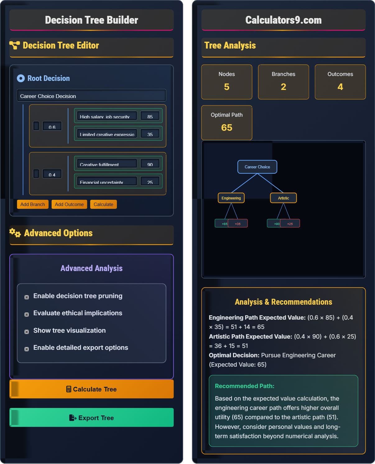
Engineering Path Expected Value: (0.6 × 85) + (0.4 × 35) = 51 + 14 = 65
Artistic Path Expected Value: (0.4 × 90) + (0.6 × 25) = 36 + 15 = 51
Optimal Decision: Pursue Engineering Career (Expected Value: 65)
Based on the expected value calculation, the engineering career path offers higher overall utility (65) compared to the artistic path (51). However, consider personal values and long-term satisfaction beyond numerical analysis.
| Path | Probability | Value | Expected Value |
|---|---|---|---|
| Engineering → High Salary | 0.6 | 85 | 51.0 |
| Engineering → Limited Expression | 0.4 | 35 | 14.0 |
| Artistic → Creative Fulfillment | 0.4 | 90 | 36.0 |
| Artistic → Financial Uncertainty | 0.6 | 25 | 15.0 |
| Decision Path | Total Expected Value | Recommendation |
|---|---|---|
| Engineering Career | 65.0 | Recommended |
| Artistic Career | 51.0 | Alternative |
Decision Tree Overview
A decision tree is a graphical representation of possible solutions to a decision based on certain conditions. It's a model of decisions and their possible consequences including chance event outcomes, resource costs, and utility. Decision trees are commonly used in operations research, specifically in decision analysis, to help identify a strategy most likely to reach a goal.
Decision trees use a tree-like model of decisions and their possible consequences. Each internal node represents a test on an attribute, each branch represents the outcome of the test, and each leaf node represents a class label or decision outcome. The paths from root to leaf represent classification rules.
- Identify all possible decision paths systematically
- Assign realistic probabilities to uncertain events
- Quantify outcomes using consistent metrics
- Calculate expected values for each path
Decision Tree Learning Quiz
Which of the following correctly identifies the three main components of a decision tree?
The answer is D) All of the above. Decision trees consist of nodes (decision points), edges (branches connecting decisions), and leaves (terminal outcomes). Alternatively, they can be described as having decisions (root and internal nodes), probabilities (on branches), and outcomes (leaf nodes). They also have a root (starting point), branches (paths), and terminal nodes (end points).
Decision trees can be understood from multiple perspectives, which is why they're so versatile in critical thinking. The structural perspective focuses on nodes and branches, the probabilistic perspective emphasizes probabilities and outcomes, and the process perspective highlights the sequence from root to terminal nodes. Understanding all perspectives helps in building and interpreting decision trees effectively.
Root Node: Starting point of the decision tree
Decision Node: Point where a choice must be made
Chance Node: Point representing uncertain outcomes
Terminal Node: End point with final outcome
• Every path must lead to a terminal node
• Probabilities of all branches from a chance node sum to 1
• Decision trees should be exhaustive of all possibilities
• Start with the root decision and work outward
• Ensure all possible outcomes are included
• Use consistent value metrics throughout
• Forgetting to include all possible outcomes
• Assigning probabilities that don't sum to 1
• Using inconsistent value scales across outcomes
Explain how to calculate the expected value of a decision path and why this calculation is important for decision making.
The expected value of a decision path is calculated by multiplying the probability of each outcome by its value (utility) and summing these products: EV = Σ(Pi × Vi). For example, if a path has two outcomes with probabilities 0.6 and 0.4 and values 85 and 35 respectively, the expected value is (0.6 × 85) + (0.4 × 35) = 51 + 14 = 65. This calculation is important because it provides a quantitative basis for comparing different decision paths, allowing for systematic evaluation of choices under uncertainty.
Expected value calculation transforms complex decision scenarios into comparable numeric values, enabling rational choice between alternatives. This mathematical approach helps overcome cognitive biases that might otherwise cloud judgment. However, it's important to remember that expected value is just one factor in decision making, and other considerations like risk tolerance and ethical implications should also be taken into account.
Expected Value: Sum of all possible outcomes weighted by their probabilities
Utility: Measure of preference or satisfaction
Uncertainty: Lack of knowledge about future outcomes
• Multiply probability by value for each outcome
• Sum all probability-value products
• Higher expected value indicates better decision
• Use consistent value scales across all outcomes
• Double-check probability sums equal 1
• Consider sensitivity analysis for key parameters
• Adding probabilities instead of multiplying by values
• Forgetting to account for all possible outcomes
• Using different value scales for different outcomes
A patient has symptoms that could indicate either condition A (probability 0.7) or condition B (probability 0.3). Treatment for A costs $5000 and is 90% effective. Treatment for B costs $8000 and is 80% effective. If treatment fails, emergency care costs $20000. Calculate the expected cost for each treatment strategy and determine the optimal approach.
Step 1: Strategy 1 - Treat for A
If A (prob 0.7): Treatment A succeeds (0.9) = $5000, Fails (0.1) = $5000 + $20000 = $25000
If B (prob 0.3): Wrong treatment, emergency care = $20000
Expected cost = 0.7×[(0.9×5000)+(0.1×25000)] + 0.3×20000 = 0.7×[4500+2500] + 6000 = 4900 + 6000 = $10,900
Step 2: Strategy 2 - Treat for B
If A (prob 0.7): Wrong treatment, emergency care = $20000
If B (prob 0.3): Treatment B succeeds (0.8) = $8000, Fails (0.2) = $8000 + $20000 = $28000
Expected cost = 0.7×20000 + 0.3×[(0.8×8000)+(0.2×28000)] = 14000 + 0.3×[6400+5600] = 14000 + 3600 = $17,600
Step 3: Optimal strategy is treating for A (lower expected cost of $10,900).
This medical example demonstrates the complexity of real-world decision trees with multiple uncertainties. The optimal decision isn't simply to treat the most likely condition, but to consider the interaction between prior probabilities, treatment effectiveness, and cost consequences. Decision trees help visualize these complex interactions and make the reasoning process transparent.
Medical Decision Tree: Decision tree applied to clinical scenarios
Expected Cost: Average cost considering all possible outcomes
Treatment Effectiveness: Probability of successful treatment
• Account for all possible outcomes and their probabilities
• Consider both direct and indirect costs
• Combine probabilities using multiplication and addition rules
• Draw the tree first to visualize all paths
• Work backwards from terminal nodes
• Verify probability sums equal 1 at each chance node
• Forgetting to account for failure scenarios
• Incorrectly combining probabilities
• Ignoring the base rate of conditions
A company must decide whether to invest $1M in a new product. Market research suggests a 60% chance of success. If successful, the project generates $3M profit. If unsuccessful, the company loses the investment. The company can also hire a consultant for $100K who has an 80% accuracy rate in predicting success. Should the company hire the consultant?
Step 1: Direct investment expected value
EV = (0.6 × $3M) + (0.4 × -$1M) = $1.8M - $0.4M = $1.4M
Step 2: With consultant (considering their prediction accuracy)
When consultant predicts success (true positive): P(predict success|actual success) = 0.8
Predicted success: P(success) = (0.8×0.6)/(0.8×0.6 + 0.2×0.4) = 0.48/0.56 = 0.857
EV if proceed after predicted success = (0.857×$3M) + (0.143×-$1M) = $2.57M - $0.143M = $2.43M
When consultant predicts failure (true negative): P(failure) = 0.857
EV if don't proceed after predicted failure = $0 (avoid loss)
Overall EV with consultant = (0.56×$2.43M) + (0.44×$0) - $0.1M = $1.36M - $0.1M = $1.26M
Step 3: Direct investment ($1.4M) > With consultant ($1.26M), so don't hire consultant.
This business example illustrates the value of information in decision making. Even though the consultant provides valuable information, the cost of obtaining that information exceeds its value in this scenario. The calculation involves conditional probability (Bayes' theorem) to determine the posterior probability of success given the consultant's prediction. This demonstrates the importance of quantifying the value of information before acquiring it.
Value of Information: Increase in expected value from obtaining additional information
Conditional Probability: Probability of an event given that another event occurred
Posterior Probability: Updated probability after considering new evidence
• Information has value only if it changes the decision
• Use Bayes' theorem to update probabilities
• Compare cost of information to its value
• Calculate value of information separately
• Use decision trees to visualize information value
• Consider both accuracy and cost of information
• Assuming all information is valuable
• Forgetting to subtract information acquisition costs
• Incorrectly applying Bayes' theorem
Which of the following is NOT a limitation of decision trees?
The answer is C) Ability to model sequential decisions. This is actually an advantage of decision trees, not a limitation. Decision trees naturally represent sequential decision-making processes where choices depend on previous decisions and chance events. The other options are genuine limitations: continuous variables need discretization, trees can overfit training data, and small changes in input can dramatically alter the tree structure.
Understanding both the capabilities and limitations of decision trees is crucial for their appropriate application. Their ability to model sequential decisions is one of their key strengths, making them ideal for multi-stage decision processes. However, practitioners must be aware of limitations like overfitting, sensitivity to data changes, and the need to discretize continuous variables to avoid misapplication.
Sequential Decisions: Decisions that depend on previous decisions and outcomes
Overfitting: Model performs well on training data but poorly on new data
Continuous Variables: Variables that can take any value within a range
• Sequential decisions are handled naturally by decision trees
• Prune trees to avoid overfitting
• Validate models on independent data
• Use cross-validation to assess overfitting risk
• Apply pruning techniques to simplify trees
• Consider ensemble methods for better performance
• Misidentifying advantages as limitations
• Overlooking the sequential nature of decisions
• Failing to validate model performance
Decision Tree FAQ
Q: How do decision trees handle ethical considerations in decision-making?
A: Decision trees can incorporate ethical considerations in several ways:
1. Value Assignment: Assign ethical weights to outcomes based on moral principles
2. Constraint Modeling: Include ethical constraints as decision nodes
3. Multi-Criteria Analysis: Evaluate decisions based on multiple ethical frameworks
4. Stakeholder Impact: Model effects on different groups
However, decision trees have limitations in capturing the nuance of ethical reasoning. They're excellent for structuring ethical dilemmas but should be combined with ethical reasoning frameworks. The quantitative approach helps identify trade-offs but doesn't resolve fundamental ethical tensions between competing values.
Q: When should I use decision trees instead of other decision-making methods?
A: Decision trees are particularly suitable when:
- Decisions involve sequential steps with uncertainty
- Multiple decision points need to be considered
- Probabilities of different outcomes can be estimated
- Outcomes can be quantified in consistent units
- Transparency in the decision process is important
They're less suitable for problems with continuous decision variables, highly correlated factors, or when the decision space is too large. For strategic decisions involving multiple stakeholders with different values, decision trees should be combined with other methods like multi-criteria decision analysis.