Regression Calculator
Fast regression analysis • 2026 edition
Regression Formula:
Show the calculatorSimple Linear Regression: \(y = mx + b\)
Slope: \(m = \frac{n(\sum xy) - (\sum x)(\sum y)}{n(\sum x^2) - (\sum x)^2}\)
Y-Intercept: \(b = \frac{\sum y - m(\sum x)}{n}\)
Correlation Coefficient: \(r = \frac{n(\sum xy) - (\sum x)(\sum y)}{\sqrt{[n\sum x^2 - (\sum x)^2][n\sum y^2 - (\sum y)^2]}}\)
Regression analysis finds the line of best fit through data points by minimizing the sum of squared residuals. The slope (m) measures the change in y for each unit change in x, and the y-intercept (b) is the value of y when x is 0.
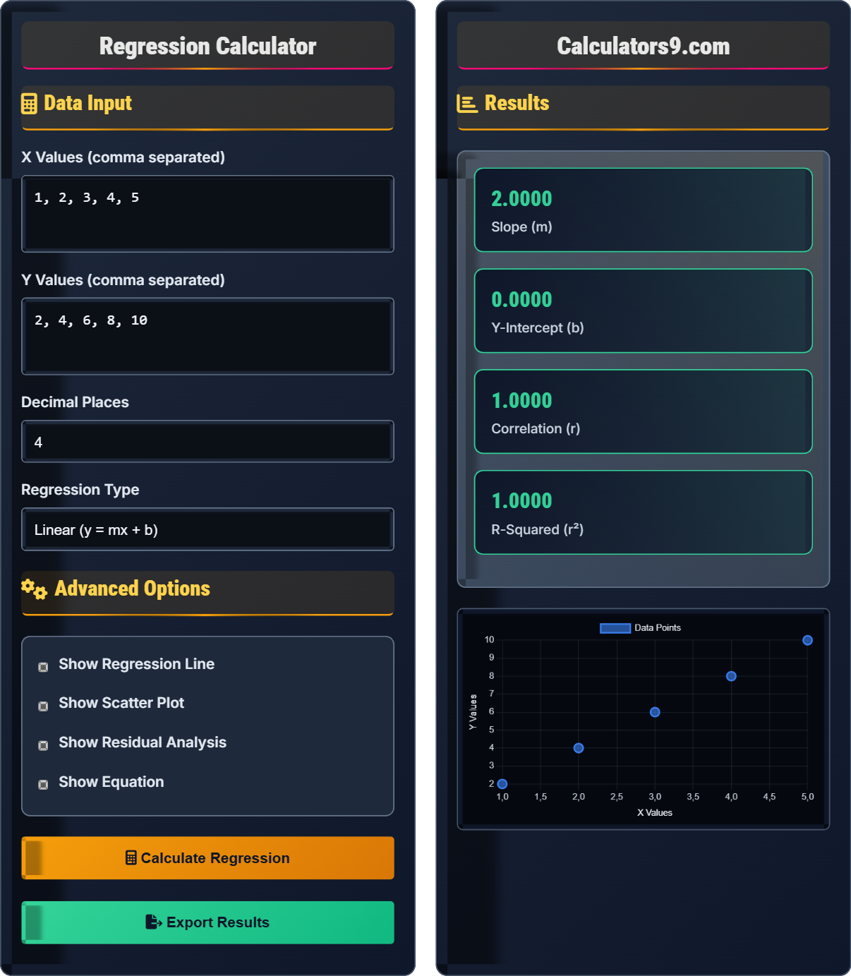
Example: For datasets X=[1, 2, 3, 4, 5] and Y=[2, 4, 6, 8, 10]:
- Sum of X: 15, Sum of Y: 30
- Sum of XY: 1×2 + 2×4 + 3×6 + 4×8 + 5×10 = 110
- Sum of X²: 1² + 2² + 3² + 4² + 5² = 55
- Slope: m = (5×110 - 15×30)/(5×55 - 15²) = (550-450)/(275-225) = 100/50 = 2
- Y-intercept: b = (30 - 2×15)/5 = 0
- Regression equation: y = 2x + 0
The correlation coefficient r = 1.0 indicates a perfect positive linear relationship.
Data Input
Advanced Options
Results
| Parameter | Value |
|---|---|
| Slope (m) | 2.0000 |
| Y-Intercept (b) | 0.0000 |
| Correlation Coefficient (r) | 1.0000 |
| Coefficient of Determination (r²) | 1.0000 |
| Standard Error | 0.0000 |
| Statistic | Value |
|---|---|
| Number of Points | 5 |
| Sum of X | 15.0000 |
| Sum of Y | 30.0000 |
| Sum of XY | 110.0000 |
| Sum of X² | 55.0000 |
Comprehensive Regression Guide
Regression analysis is a statistical method used to model the relationship between a dependent variable (Y) and one or more independent variables (X). Simple linear regression fits a straight line to data points that minimizes the sum of squared differences between observed and predicted values. The goal is to predict the value of Y based on X values.
The simple linear regression equation is:
\(y = mx + b\)
Where:
- \(y\) = dependent variable
- \(x\) = independent variable
- \(m\) = slope of the line
- \(b\) = y-intercept
The slope and intercept are calculated using:
The coefficient of determination (r²) represents the proportion of variance in the dependent variable that is predictable from the independent variable. It ranges from 0 to 1, where 1 indicates perfect prediction. For example, r² = 0.85 means 85% of the variation in Y can be explained by X.
- Economics: Predicting sales based on advertising spend
- Medicine: Modeling drug effectiveness vs dosage
- Engineering: Reliability analysis and quality control
- Psychology: Predicting behavior from personality traits
Regression Concepts
Statistical method to model relationship between variables.
Minimizes sum of squared residuals.
Standard approach for finding best-fit line.
- Assumes linear relationship
- Minimizes squared errors
- Requires paired data
Advanced Concepts
Difference between observed and predicted values.
Check for patterns in residuals.
- Random scatter = good fit
- Patterns = model inadequacy
- Constant variance = homoscedasticity
- Correlation does not imply causation
- Extrapolation beyond data range risky
- Outliers can strongly influence results
Regression Learning Quiz
What does the coefficient of determination (r²) measure in regression analysis?
The answer is B) The proportion of variance in Y explained by X. The coefficient of determination (r²) specifically measures the proportion of the variance in the dependent variable (Y) that is predictable from the independent variable (X). For example, if r² = 0.75, then 75% of the variation in Y can be explained by the variation in X. It is calculated as the square of the correlation coefficient (r) and ranges from 0 to 1.
This question tests the fundamental understanding of what r² represents. Students often confuse r² with the correlation coefficient r itself. While r measures the strength and direction of the linear relationship, r² measures the proportion of explained variance. Both are important but measure different aspects of the relationship.
Explained variance: Variation in Y accounted for by X
Total variance: Overall variation in the dependent variable
Proportion: Fraction of total variance explained
• r² ranges from 0 to 1
• Higher values indicate better fit
• r² = 1 means perfect prediction
• r² is always positive
• Multiply by 100 to get percentage
• Compare r² values to assess models
• Confusing r² with correlation coefficient r
• Interpreting r² as causation
• Expecting r² to always be close to 1
Calculate the regression equation for the following data: X = [1, 2, 3, 4, 5] and Y = [2, 4, 6, 8, 10]. Show all steps of the calculation.
Step 1: Calculate the required sums
n = 5 (number of data points)
ΣX = 1 + 2 + 3 + 4 + 5 = 15
ΣY = 2 + 4 + 6 + 8 + 10 = 30
ΣXY = (1×2) + (2×4) + (3×6) + (4×8) + (5×10) = 2 + 8 + 18 + 32 + 50 = 110
ΣX² = 1² + 2² + 3² + 4² + 5² = 1 + 4 + 9 + 16 + 25 = 55
Step 2: Calculate the slope (m)
m = [n(ΣXY) - (ΣX)(ΣY)] / [n(ΣX²) - (ΣX)²]
m = [5(110) - (15)(30)] / [5(55) - (15)²]
m = [550 - 450] / [275 - 225]
m = 100 / 50 = 2
Step 3: Calculate the y-intercept (b)
b = [ΣY - m(ΣX)] / n
b = [30 - 2(15)] / 5
b = [30 - 30] / 5 = 0
Step 4: Write the regression equation
y = mx + b
y = 2x + 0
y = 2x
Step 5: Verify the equation
For x=1: y = 2(1) = 2
For x=2: y = 2(2) = 4 ✓
For x=3: y = 2(3) = 6 ✓
For x=4: y = 2(4) = 8 ✓
For x=5: y = 2(5) = 10 ✓
Final Answer: The regression equation is y = 2x, with slope m = 2 and y-intercept b = 0.
This calculation demonstrates the systematic approach to finding the least squares regression line. The key insight is that the formulas for slope and intercept are derived to minimize the sum of squared residuals. In this example, the perfect linear relationship (r=1.0) results in all points lying exactly on the regression line.
Least squares: Method that minimizes squared errors
Residual: Difference between observed and predicted valuesSum of squares: Sum of squared deviations
• Always calculate sums first
• Substitute values carefully
• Verify with sample points
• Create a table to organize calculations
• Double-check arithmetic operations
• Graph the line to verify fit
• Arithmetic errors in calculations
• Using wrong formula components
• Forgetting to square values in ΣX²
FAQ
Q: What is the difference between correlation and regression?
A: While correlation and regression are related, they serve different purposes:
Correlation: Measures the strength and direction of a linear relationship between two variables. The correlation coefficient (r) ranges from -1 to +1 and indicates how closely the variables move together. It doesn't distinguish between dependent and independent variables.
Regression: Models the relationship between variables to predict one variable based on another. It produces an equation (like y = mx + b) that can be used to make predictions. It explicitly identifies one variable as dependent and another as independent.
In essence, correlation answers "how strong is the relationship?" while regression answers "what is the equation of the relationship?" Correlation is symmetric (switching X and Y doesn't change r), but regression is not (switching X and Y gives different equations).
Q: How do I interpret residuals in regression analysis?
A: Residuals are the differences between observed values and values predicted by the regression model (residual = observed - predicted). They provide crucial diagnostic information:
Good Model: Residuals should be randomly scattered around zero with no discernible pattern. This indicates that the model captures the underlying relationship well.
Problems Indicated by Patterns:
- Curved pattern suggests non-linearity
- Fanning pattern indicates heteroscedasticity (non-constant variance)
- Systematic trend suggests missing variables
Residual analysis is essential for validating regression assumptions. A residual plot (residuals vs fitted values) is a powerful tool for identifying violations of assumptions like linearity, constant variance, and independence.